Consider moving / teaching this BEFORE geometric pose estimation. It could actually be nice to introduce cameras / point clouds with this material instead of with pose estimation.
In this chapter we'll consider the simplest version of the bin picking
problem: the robot has a bin full of random objects and simply needs to move
those objects from one bin to the other. We'll be agnostic about what those
objects are and about where they end up in the other bin, but we would like
our solution to achieve a reasonable level of performance for a very wide
variety of objects. This turns out to be a pretty convenient way to create a
training ground for robot learning -- we can set the robot up to move objects
back and forth between bins all day and night, and intermittently add and
remove objects from the bin to improve diversity. Of course, it is even
easier in simulation!
Bin picking has potentially very important applications in industries such
as logistics, and there are significantly more refined versions of this
problem. For example, we might need to pick only objects from a specific
class, and/or place the objects in known position (e.g. for "packing"). But
let's start with the basic case.
Generating random cluttered scenes
If our goal is to test a diversity of bin picking situations, then the
first task is to figure out how to generate diverse simulations. How
should we populate the bin full of objects? So far we've set up each
simulation by carefully setting the initial positions (in the
Context) for each of the objects, but that approach won't
scale.
Falling things
In the real world, we would probably just dump the random objects into
the bin. That's a decent strategy for simulation, too. We can roughly
expect our simulation to faithfully implement multibody physics as long
as our initial conditions (and time step) are reasonable; but the physics
isn't well defined if we initialize the Context with
multiple objects occupying the same physical space. The simplest and
most common way to avoid this is to generate a random number of objects
in random poses, with their vertical positions staggered so that they
trivially start out of penetration.
If you look for them, you can find animations of large numbers of
falling objects in the demo reels for most advanced multibody simulators.
(These demos can potentially be a bit misleading; it's relatively easy to
make a simulation which lots of objects falling that looks relatively
good from a distance, but if you zoom in and look closely you'll often
find many anomalies.) For our purposes the falling dynamics themselves
are not the focus. We just want the state of the objects when they are
done falling as initial conditions for our manipulation system.
maybe cite the falling things paper, but make it clear that the idea
is not new?
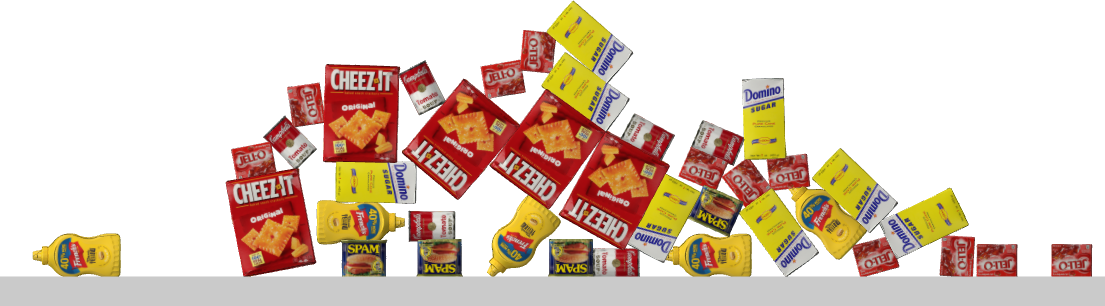
Piles of foam bricks in 2D
Here is the 2D case. I've added many instances of our favorite red
foam brick to the plant. Note that it's possible to write highly
optimized simulators that take advantage of physics being restricted to
2D; that's not what I've done here. Rather, I've added a planar joint
connecting each brick to the world, and run our full 3D simulator. The
planar joint has three degrees of freedom. I've oriented them here to
be $x$, $z$, and $\theta$ to constrain the objects to the $xz$
plane.
I've set the initial positions for each object in the
Context to be uniformly distributed over the horizontal
position, uniformly rotated, and staggered every 0.1m in their initial
vertical position. We only have to simulate for a little more than a
second for the bricks to come to rest and give us our intended "initial
conditions".
It's not really any different to do this with any random objects --
here is what it looks like when I run the same code, but replace the
brick with a random draw from a few objects from the YCB dataset
Calli17. It somehow amuses me that we can see the central limit
theorem hard at work, even when our objects are slightly
ridiculous.
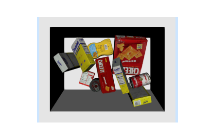
Filling bins with clutter
The same technique also works in 3D. Setting uniformly random
orientations in 3D requires a little more thought, but Drake supplies
the method UniformlyRandomRotationMatrix (and also one for
quaternions and roll-pitch-yaw) to do that work for us.
Please appreciate that bins are a particularly simple case for
generating random scenarios. If you wanted to generate random kitchen
environments, for example, then you won't be as happy with a solution
that drops refrigerators, toasters, and stools from uniformly random
i.i.d. poses. In those cases, authoring reasonable distributions gets
much more interesting Izatt20; we will revisit the topic of
generative scene models later in the notes.
Static equilibrium with frictional contact
Although the examples above are conceptually very simple, there is
actually a lot going on in the physics engine to make all of this work.
To appreciate a few of the details, let's explore the easiest case -- the
(static) mechanics once all of the objects have come to rest.
I won't dive into a full discussion of multibody dynamics nor multibody
simulation, though I do have more notes available here. What
is important to understand is that the familiar $f=ma$ takes a particular
form when we write it down in terms of the generalized positions, $q$, and
velocities, $v$: $$M(q)\dot{v} + C(q,v)v = \tau_g(q) + \sum_i
J^T_i(q)F^{c_i}.$$ We already understand the generalized positions, $q$,
and velocities, $v$. The left side of the equation is just a generalization
of "mass times acceleration", with the mass matrix, $M$, and the Coriolis
terms $C$. The right hand side is the sum of the (generalized) forces, with
$\tau_g(q)$ capturing the terms due to gravity, and $F^{c_i}$ is the
spatial force due to the $i$th contact. $J_i(q)$ is the $i$th "contact
Jacobian" -- it is the Jacobian that maps from the generalized velocities
to the spatial velocity of the $i$th contact frame.
Our interest here is in finding (stable) steady-state solutions to
these differential equations that can serve as good initial conditions
for our simulation. At steady-state we have $v=\dot{v}=0$, and
conveniently all of the terms on the left-hand side of the equations are
zero. This leaves us with just the force-balance equations $$\tau_g(q) =
- \sum_i J^T_i(q) F^{c_i}.$$
Spatial force
Before we proceed, let's be a little more careful about our force
notation, and define its spatial algebra. Often we think of forces as a
three-element vector (with components for $x$, $y$, and $z$) applied to a
rigid body at some point. More generally, we will define a six-component
vector for spatial
force, using the monogram notation:
\begin{equation}F^{B_p}_{{\text{name}},C} = \begin{bmatrix}
\tau^{B_p}_{\text{name},C} \\ f^{B_p}_{\text{name},C} \end{bmatrix} \quad
\text{ or, if you prefer } \quad \left[F^{B_p}_{\text{name}}\right]_C =
\begin{bmatrix} \left[\tau^{B_p}_{\text{name}}\right]_C \\
\left[f^{B_p}_{\text{name}}\right]_C \end{bmatrix}.\end{equation}
$F^{B_p}_{\text{name},C}$ is the named spatial force applied to a point,
or frame origin, $B_p$, expressed in frame $C$. The form with the
parentheses is preferred in Drake, but is a bit too verbose for my taste
here in the notes. The name is optional, and the expressed in frame, if
unspecified, is the world frame. For forces in particular, it is
recommended that we include the body, $B$, that the force is being
applied to in the symbol for the point $B_p$, especially since we will
often have equal and opposite forces. In code, we write
Fname_Bp_C.
Like spatial velocity, spatial forces have a rotational component and
a translational component; $\tau^{B_p}_C \in \Re^3$ is the torque
(on body $B$ applied at point $p$ expressed in frame $C$), and
$f^{B_p}_C \in \Re^3$ is the translational or Cartesian force. A
spatial force is also commonly referred to as a wrench. If
you find it strange to think of forces as having a rotational
component, then think of it this way: the world might only impart
Cartesian forces at the points of contact, but we often want to
summarize the combined effect of many Cartesian forces applied to
different points into one common frame. To do this, we represent the
equivalent effect of each Cartesian force at the point of application
as a force
and a torque applied at a different point on the body.
Spatial forces fit neatly into our spatial algebra:
Spatial forces add when they are applied to the same body in the
same frame, e.g.: \begin{equation}F^{B_p}_{\text{total},C}
= \sum_i F^{B_p}_{i,C} .\end{equation}
Shifting a spatial force from one application point, $B_p$, to
another point, $B_q$, uses the cross product: \begin{equation} f^{B_q}_C
= f^{B_p}_C, \qquad \tau^{B_q}_C = \tau^{B_p}_C + {}^{B_q}p^{B_p}_C
\times f^{B_p}_C.\label{eq:spatial_force_shift}\end{equation}
As with all spatial vectors, rotations can be used to change
between the "expressed-in" frames: \begin{equation} f^{B_p}_D = {}^DR^C
f^{B_p}_C, \qquad \tau^{B_p}_D = {}^DR^C
\tau^{B_p}_C.\end{equation}
Collision geometry
Now that we have our notation, we next need to understand where the
contact forces come from.
Geometry engines for robotics, like SceneGraph in
, distinguish between a few different roles
that geometry can play in a simulation. In robot description files, we
distinguish between visual
and collision
geometries. In particular, every rigid body in the simulation can have
multiple
collision
geometries associated with it (playing the "proximity" role). Collision
geometries are often much simpler than the visual geometries we use for
illustration and simulating perception -- sometimes they are just a
low-polygon-count version of the visual mesh and sometimes we actually
use much simpler geometry (like boxes, spheres, and cylinders). These
simpler geometries make the physics engine faster and more robust.
Collision geometry inspector
Drake has a very useful ModelVisualizer tool that
publishes by the illustration and collision geometry roles to Meshcat
(see, for example, the Drake ). This is very useful for designing new models, but also for
understanding the contact geometry of existing models.
We used this tool before, when we were visualizing the various robot
models. Go ahead and try it again; navigate in the meshcat controls to
Scene > drake > proximity and check the box to enable
visualizing the geometries with the proximity role.
Visualizing the visual and collision geometries for the
UR3e.
SceneGraph also implements the concept of a collision
filter. It can be important to specify that, for instance, the iiwa
geometry at link 5 cannot collide with the geometry in links 4 or 6.
Specifying that some collisions should be ignored not only speeds up the
computation, but it also facilitates the use of simplified collision
geometry for links. It would be extremely hard to approximate link 4 and
5 accurately with spheres, and cylinders if I had to make sure that those
spheres and cylinders did not overlap in any feasible joint angle. The
default collision filter settings should work fine for most applications,
but you can tweak them if you like.
So where do the contact forces, $f^{c_i}$, come from? There is
potentially an equal and opposite contact (spatial) force for every
pair of collision geometries that are not filtered out by the
collision filter. In SceneGraph, the GetCollisionCandidates
method returns them all. We'll take to calling the two bodies in a collision pair "body A" and "body B".
Contact forces between bodies in collision
In our mathematical models, two bodies would never occupy the same
region of space, but in a simulation using numerical integration, this can
rarely be avoided completely. Most simulators summarize the contact forces
between two bodies that are in collision -- either touching or overlapping
-- as Cartesian forces at one or more contact points. It's easy to
underestimate this step!
First, let's appreciate the sheer number of cases that we have to get right in
the code; it's unfortunately extremely common for open-source tools to have bugs in
here. But I think the simple gui I've created below makes it pretty apparent that
asking to summarize the forces between two bodies in deep penetration with a single
Cartesian force applied at a point is fraught with peril. As you move the objects,
you will find many discontinuities; this is a common reason why you sometimes see
rigid body simulations "explode". It might seem natural to try to use multiple
contact points instead of a single contact point to summarize the forces, and some
simulators do, but it is very hard to write an algorithm that only depends on the
current configurations of the geometry which selects contact points consistently
from one time step to the next.
One of the innovations in Drake which makes it particularly good at simulating complex contact situations is that we have moved away from point contact models. When we enable hydroelastic contact in Drake, the spatial forces between two penetrating bodies are computed by taking an integral over a "hydroelastic surface" which generalizes the notion of a contact patch Elandt19. As of this writing, you still have to "opt-in" to using hydroelastic in Drake (see ); I'm working to use it in all of my examples in these notes.
More about hydroelastic here. Show some of the nice videos.
https://youtu.be/5-k2Pc6OmzE
Contact force inspector
I've created a simple GUI that allows you to pick any two primitive
geometry types and inspect the hydroelastic contact information that is
computed when those object are put into penetration.
The Contact Frame
We still need to decide the magnitude and direction of these spatial
forces, and to do this we need to specify the
contact frame in which the spatial force is to be applied. For
instance, we might
use $C_B$ to denote a contact frame on body $B$, with the forces
applied at the origin of the frame.
Although I strongly advocate for using the hydroelastic contact model in
your simulations, for the purposes of exposition, let's think about the
point contact model here. If the collision engine produces a number of
contact point locations, how should we define the frames?
Our convention will be to align the positive $z$ axis with the "contact
normal", with positive forces resisting penetration. Defining this normal
also requires care. For instance, what is the normal at the corner of a
box? Taking the normal as a (sub-)gradient of the
signed-distance function between two bodies provides a reliable definition
that will extend into generalized coordinates. The $x$ and $y$ axes of the
contact frame are any orthogonal basis for the tangential coordinates. You
can find additional figures and explanations here.
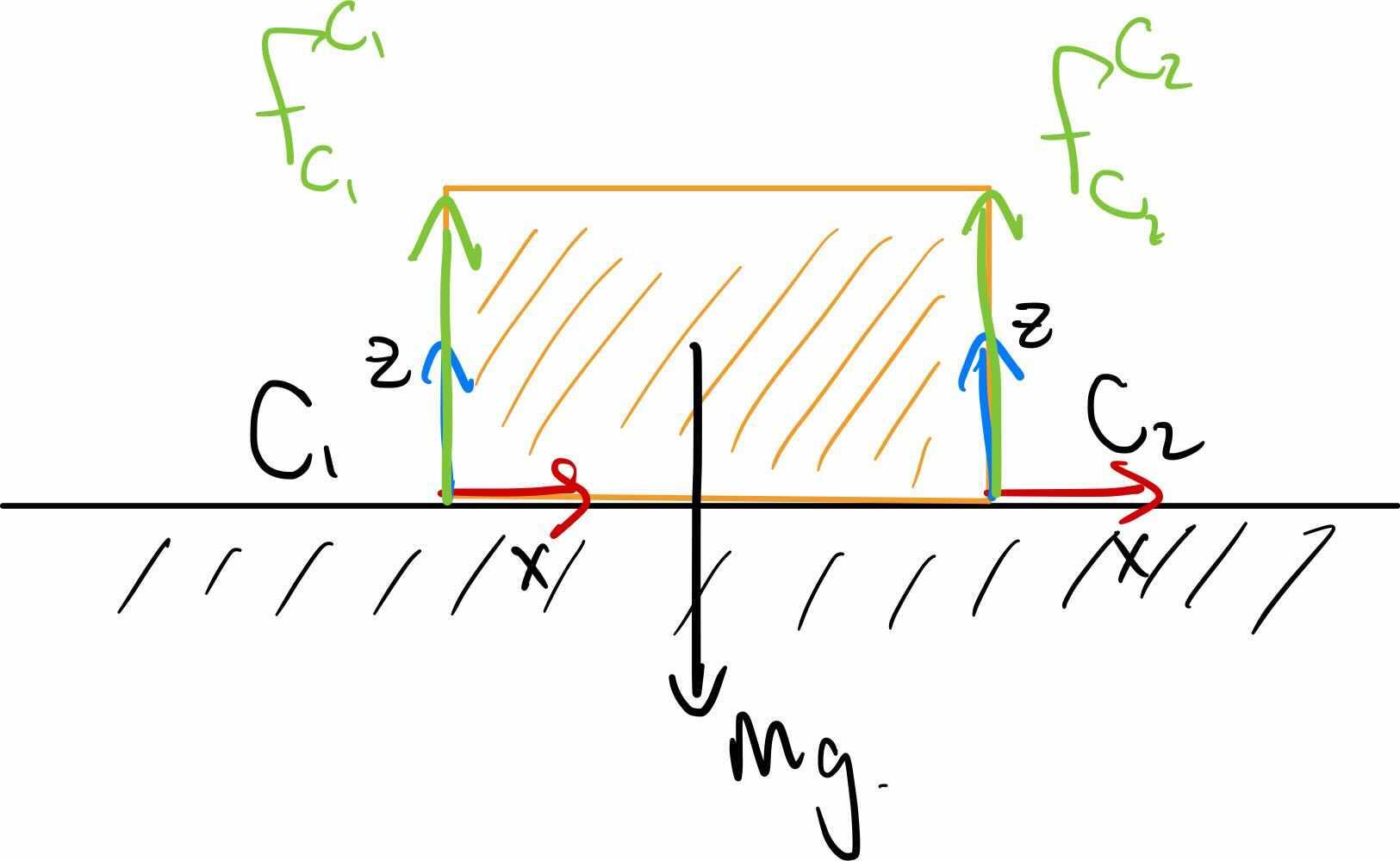
Brick on a half-plane
Let's work through these details on a simple example -- our foam
brick sitting on the ground. The ground is welded to the world, so has
no degrees of freedom; we can ignore the forces applied to the ground
and focus on the forces applied to the brick.
Where are the contact forces and contact frames? If we used only
box-on-box geometry, then the choice of contact force location is not
unique during this "face-on-face" contact; this is even more true in 3D
(where three forces would be sufficient). Let's assume for a moment
that our contact engine determines two points of contact -- one at each
corner of the box. (In order to help the contact engine make robust
choices when we are using point contact models, we sometimes actually
annotate the boxes with
small sphere collision geometries in the eight corners; this is not
needed when using hydroelastic contact.) I've labeled the frames $C_1$
and $C_2$ in the sketch below.
In order to achieve static equilibrium, we require that all of the
forces and torques on the brick be in balance. We have three forces to
consider: $F_{g}, F_1,$ and $F_2$, named using shorthand for gravity,
contact 1, and contact 2, respectively. The gravity vector is most
naturally described in the world frame, applied to the body at the center
of mass: $$F_{g, W}^B = \begin{bmatrix} 0, 0, 0, 0, 0, -mg
\end{bmatrix}^T.$$ The contact forces are most naturally described in the
contact frames; for instance we know that $$f_{1, C_1,z}^{B_{c_1}} \ge
0,$$ because the force cannot pull on the ground. To write the force
balance equation, we need to use our spatial algebra to express all of
the spatial forces in the same frame, and apply them at the same
point.
For instance, if we are to transform contact force 1, we can first
change the frame: $$F_{1,B}^{B_{c_1}} = {}^B R^{C_1}
F_{1,C_{1}}^{B_{c_1}}.$$ Then we can change the point at which it's
applied: $$f_{1,B}^B = f_{1,B}^{B_{c_1}}, \qquad \tau_{1,B}^B =
\tau_{1,B}^{B_{C_1}} + {}^Bp_B^{B_{C_1}} \times f_{1,B}^{B_{c_1}}.$$ We
can now solve for the force balance: $$F_{1,B}^B + F_{2,B}^B + F_{g,B}^B
= 0,$$ which is six equations in 3D (or only three in 2D). The
translational components tell me that $$f_{1,B}^B + f_{2,B}^B =
\begin{bmatrix}0 \\ 0 \\ mg\end{bmatrix},$$ but it's the torque
component in $y$ that tells me that $f_{1,B_z}$ and $f_{2,B_z}$ must be
equal if the center of mass is equally distance from the two contact
points.
We haven't said anything about the horizontal
forces yet, except that they must balance. Let's develop that
next.
The (Coulomb) Friction Cone
Now the rules governing contact forces can begin to take shape. First
and foremost, we demand that there is no force at a distance. Using
$\phi_i(q)$ to denote the distance between two bodies in configuration
$q$, we have $$\phi(q) > 0 \Rightarrow f^{c_i} = 0.$$ Second, we demand
that the normal force only resists penetration; bodies are never pulled
into contact: $$f^{c_i}_{C_z} \ge 0.$$ In rigid contact models, we
solve for the smallest normal force that enforces the non-penetration
constraint (this is known as the principle of least constraint). In
soft contact models, we define the force to be a function of the
penetration depth and velocity.
CitationsNeed figures here
Forces in the tangential directions are due to friction. The most
commonly used model of friction is Coulomb friction, which states that
$$\sqrt{{f^{c_i}_{C_x}}^2 + {f^{c_i}_{C_y}}^2} \le \mu f^{c_i}_{C_z},$$ with $\mu$ a
non-negative scalar coefficient of friction. Typically we define
both $\mu_{static}$, which is applied when the tangential velocity is
zero, and $\mu_{dynamic}$, applied when the tangential velocity is
non-zero. In the Coulomb friction model, the tangential contact force is
the force within this friction cone which produces maximum dissipation.
Taken together, the geometry of these constraints forms a cone of admissable
contact forces. It is famously known as the "friction cone", and we will
refer to it often.
It's a bit strange for us to write that the forces are in some set.
Surely the world will pick just one force to apply? It can't apply all
forces in a set. The friction cone specifies the range of possible
forces; under the Coulomb friction model we say that the one force that
will be picked is the force inside this set that will successfully resist
relative motion in the contact x-y frame. If no force inside the friction
cone can completely resist the motion, then we have sliding, and we say
that the force that the world will apply is the force inside the friction
cone of maximal dissipation. For the conic friction cone, this
will be pointed in the direction opposite of the sliding velocity. So
even though the world will indeed "pick" one force from the friction cone
to apply, it can still be meaningful to reason about the set of possible
forces that could be applied because those denote the set of possible
opposing forces that friction can perfectly resist. For instance, a brick
under gravity will not move if we can exactly oppose the force of gravity
with a force inside the friction cone.
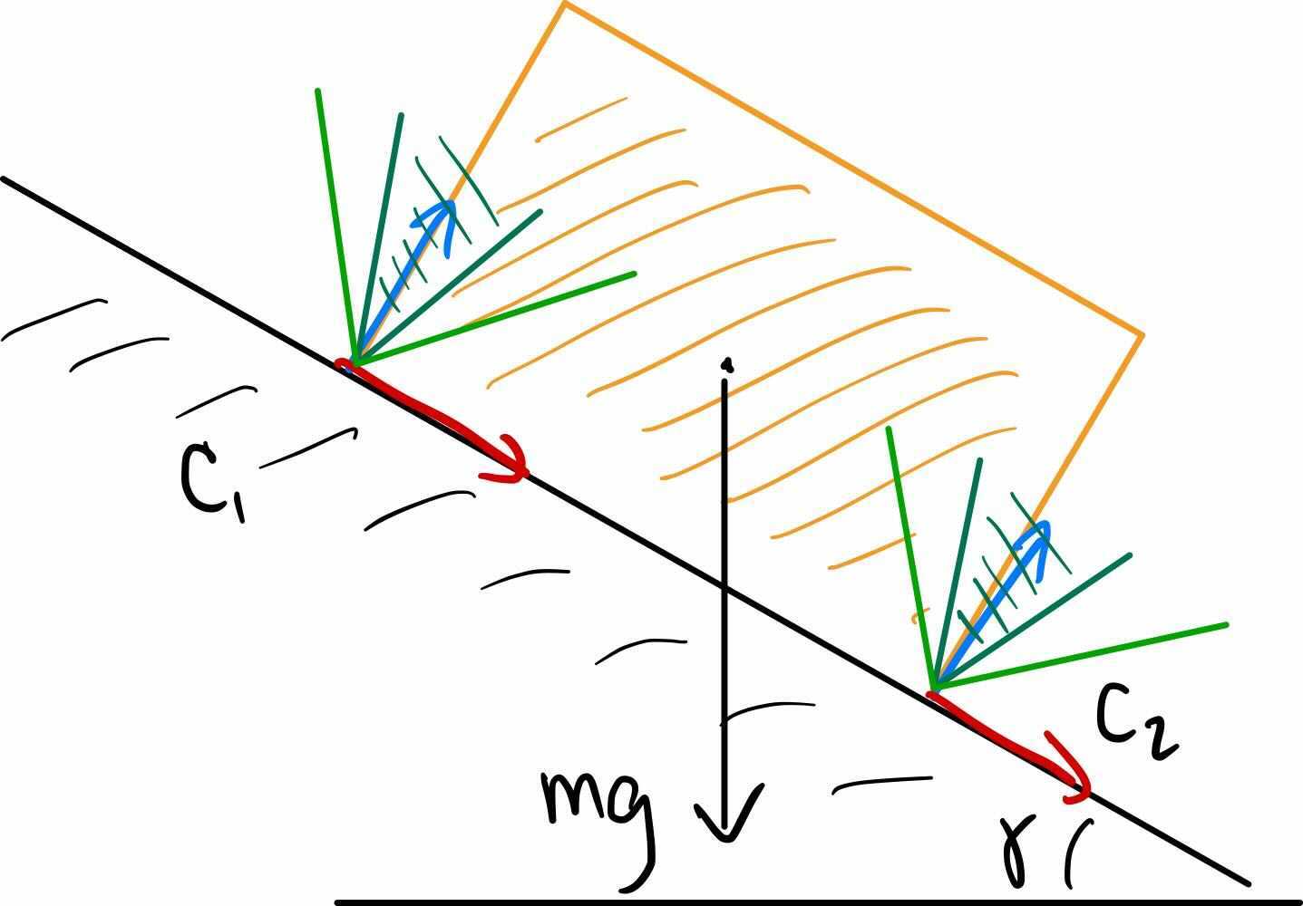
Brick on an inclined half-plane
If we take our last example, but tilt the table to an angle relative
to gravity, then the horizontal forces start becoming important.
Before going through the equations, let's check your intuition. Will
the magnitude of the forces on the two corners stay the same in this
configuration? Or will there be more contact force on the lower
corner?
In the illustration above, you'll notice that the contact frames
have rotated so that the $z$ axis is aligned with the contact normals.
I've sketched two possible friction cones (dark green and lighter
green), corresponding to two different coefficients of friction. We
can tell immediately by inspection that the smaller value of $\mu$
(corresponding to the darker green) cannot produce contact forces that
will completely counteract gravity (the friction cone does not contain
the vertical line). In this case, the box will slide and no static
equilibrium exists in this configuration.
If we increase the coefficient of (static) friction to the range
corresponding to the lighter green, then we can find contact forces that
produce an equilibrium. Indeed, for this problem, we need some amount of
friction to even have an equilibrium (we'll explore this in the exercises). We also need for the vertical
projection of the center of mass onto the ramp to land between the two
contact points, otherwise the brick will tumble over the bottom edge. We
can see this by writing our same force/torque balance equations. We can
write them applied at and expressed in body frame, B, assuming the center
of mass in the center of the brick and the brick has length $l$ and
height $h$:\begin{gather*} f^{B}_{1, B_x} + f^{B}_{2, B_x} =
-mg\sin\gamma \\ f^{B}_{1,B_z} + f^{B}_{2,B_z} = mg\cos\gamma \\ -h
f^{B}_{1,B_x} + l f^{B}_{1,B_z} = h f^{B}_{2,B_x} + l f^{B}_{2, B_z} \\
f^{B}_{1, B_z} \ge 0, \quad f^{B}_{2, B_z} \ge 0 \\ |f^{B}_{1, B_x}| \le
\mu f^{B}_{1, B_z}, \quad |f^{B}_{2, B_x}| \le \mu f^{B}_{2, B_z}
\end{gather*}
So, are the magnitude of the contact forces the same or different?
Substituting the first equation into the third reveals $$f^{B}_{2, B_z}
= f^{B}_{1, B_z} + \frac{mgh}{l}\sin\gamma.$$
Static equilibrium as an optimization problem
Rather than dropping objects from a random height, perhaps we can
initialize our simulations using optimization to find the initial
conditions that are already in static equilibrium. In ,
the
StaticEquilbriumProblem
collects all of the constraints we enumerated above into an optimization
problem: \begin{align*} \find_q \quad \subjto \quad& \tau_g(q) = - \sum_i
J^T_i(q) f^{c_i} & \\ & f^{c_i}_{C_z} \ge 0 & \forall i, \\ &
|f^{c_i}_{C_{x,y}}|_2 \le \mu f^{c_i}_{C_z} & \forall i, \\ & \phi_i(q)
\ge 0 & \forall i, \\ & \phi(q) = 0 \textbf{ or } f^{c_i}_{C_z} = 0
&\forall i, \\ & \text{joint limits}.\end{align*} This is a nonlinear
optimization problem: it includes the nonconvex non-penetration
constraints we discussed in the last chapter. The second-to-last
constraints (a logical or) is particularly interesting; constraints of
the form $x \ge 0, y \ge 0, x =0 \textbf{ or } y = 0$ are known as
complementarity constraints, and are often written as $x \ge 0, y \ge 0,
xy = 0$. We can make the problem easier for the nonlinear optimization
solver by relaxing the equality to $0 \le \phi(q) f^{c_i}_{C_z} \le
\text{tol}$, which provides a proper gradient for the optimizer to follow
at the cost of allowing some force at a distance.
It's easy to add additional costs and constraints; for initial
conditions we might use an objective that keeps $q$ close to an initial
configuration-space sample.
Tall Towers
So how well does it work?
finish this...
Contact simulation
Static equilibrium problems provide a nice view into a few of the
complexities of contact simulation. But things get a lot more interesting
when the robot and/or objects in the scene start moving!
More coming soon!
Why is multibody plant discrete time?Stiff differential equations / choosing your time stepWhat makes a fast simulator?Call out to Drake's soft sim.
Model-based grasp selection
What makes a good grasp? This topic has been studied extensively for
decades in robotics, with an original focus on thinking of a (potentially
dexterous) hand interacting with a known object.
Prattichizzo08 is an excellent survey of that literature; I
will summarize just a few of the key ideas here.
If the goal of a grasp is to stabilize an object in the hand, then one
definition of a "good grasp" is be one that is able to resist
disturbances described by an "adversarial" wrench applied to the body.
The contact wrench cone
Above, we introduced the friction cone as the range of possible forces
that friction is able to produce in order to resist motion. For the
purposes of grasp planning, by applying the additive inverse to the
forces in the friction cone, we can obtain all of the "adversarial"
forces that can be resisted at the point of contact. And to understand
the total ability of all contact forces (applied at multiple points of
contact) to resist motion of the body, we want to somehow add all of
these forces together. Fortunately, the spatial algebra for spatial
forces can be readily extended from operating on spatial force vectors to
operating on entire sets of spatial forces.
Because our sets of interest here are convex cones, I will use the
relatively standard choice of $\mathcal{K}$ for the six-dimensional
wrench cone. Specifically, we have
$\mathcal{K}^{B_p}_{\text{name}, C}$ for the cone corresponding to
potential spatial forces for $F^{B_p}_{\text{name}, C}$. For instance,
our Coulomb friction cone for the point contact model (which, as we've
defined it, has no torsional friction) in the contact frame could be:
\begin{equation}\mathcal{K}^C_C = \left\{ \begin{bmatrix} 0 \\ 0 \\ 0 \\
f^{C}_{C_x} \\ f^C_{C_y} \\ f^C_{C_z} \end{bmatrix} : \sqrt{
\left(f^{C}_{C_x}\right)^2 + \left(f^{C}_{C_y}\right)^2 } \le \mu
f^C_{C_z} \right\}.\end{equation}
The spatial algebra for spatial forces can be applied directly to the
wrench cones:
For addition of wrenches applied at the same point and expressed
in the same frame, the interpretation we seek is that the cone formed
by the sum of wrench cones describes the set of wrenches that could
be obtained by choosing one element from each of the individual cones
and summing them up. This set operator is the Minkowski
sum, which we denote with $\oplus$, e.g.:
\begin{equation}\mathcal{K}^{B_p}_{\text{total},C}=
\mathcal{K}^{B_p}_{0,C} \oplus \mathcal{K}^{B_p}_{1,C} \oplus
\cdots\end{equation}
Shifting a wrench cone from one application frame, $B_p$, to
another frame, $B_q$, is a linear operation on the cones; to
emphasize that I will write Eq $\ref{eq:spatial_force_shift}$ in
matrix form: \begin{equation} \mathcal{K}^{B_q}_C = \begin{bmatrix}
I_{3 \times 3} & \left[ {}^{B_q}p^{B_p}_C \right]_\times \\ 0_{3
\times 3} & I_{3 \times 3} \end{bmatrix}
\mathcal{K}^{B_p}_C,\end{equation} where the notation $[p]_{\times}$
is the skew-symmetric matrix corresponding to the cross product.
Rotations can be used to change between the "expressed-in"
frames: \begin{equation} \mathcal{K}^{B_p}_D = \begin{bmatrix} {}^DR^C
& 0_{3 \times 3} \\ 0_{3 \times 3} & {}^DR^C \end{bmatrix}
\mathcal{K}^{B_p}_C.\end{equation}
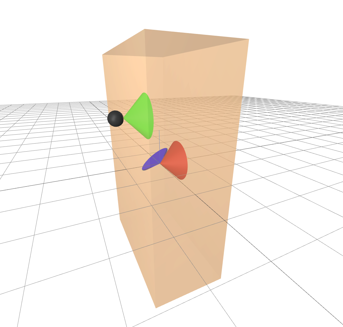
A contact wrench cone visualization
I've made a simple interactive visualization for you to play with to
help your intuition about these wrench cones. I have a box that fixed
in space and only subjected to contact forces (no gravity is
illustrated here); I've drawn the friction cone at the point of contact
and at the center of the body. Note that I've intentionally disabled
hydroelastic contact for this example -- the forces are computed using
only a single contact point between each collision pair -- to simplify
the interpretation.
There is one major caveat: the wrench cone lines in $\Re^6$, but I
can only draw cones in $\Re^3$. So I've made the (standard) choice to
draw the projection of the 6d cone into 3d space with two cones: one
for the translational components (in green for the contact point and
again in red for the body frame) and another for the rotational
components (in blue for the body frame). This can be slightly
misleading because one cannot actually select independently from both
sets.
Here is the contact wrench cone for a single contact point, visualized for two different contact locations:
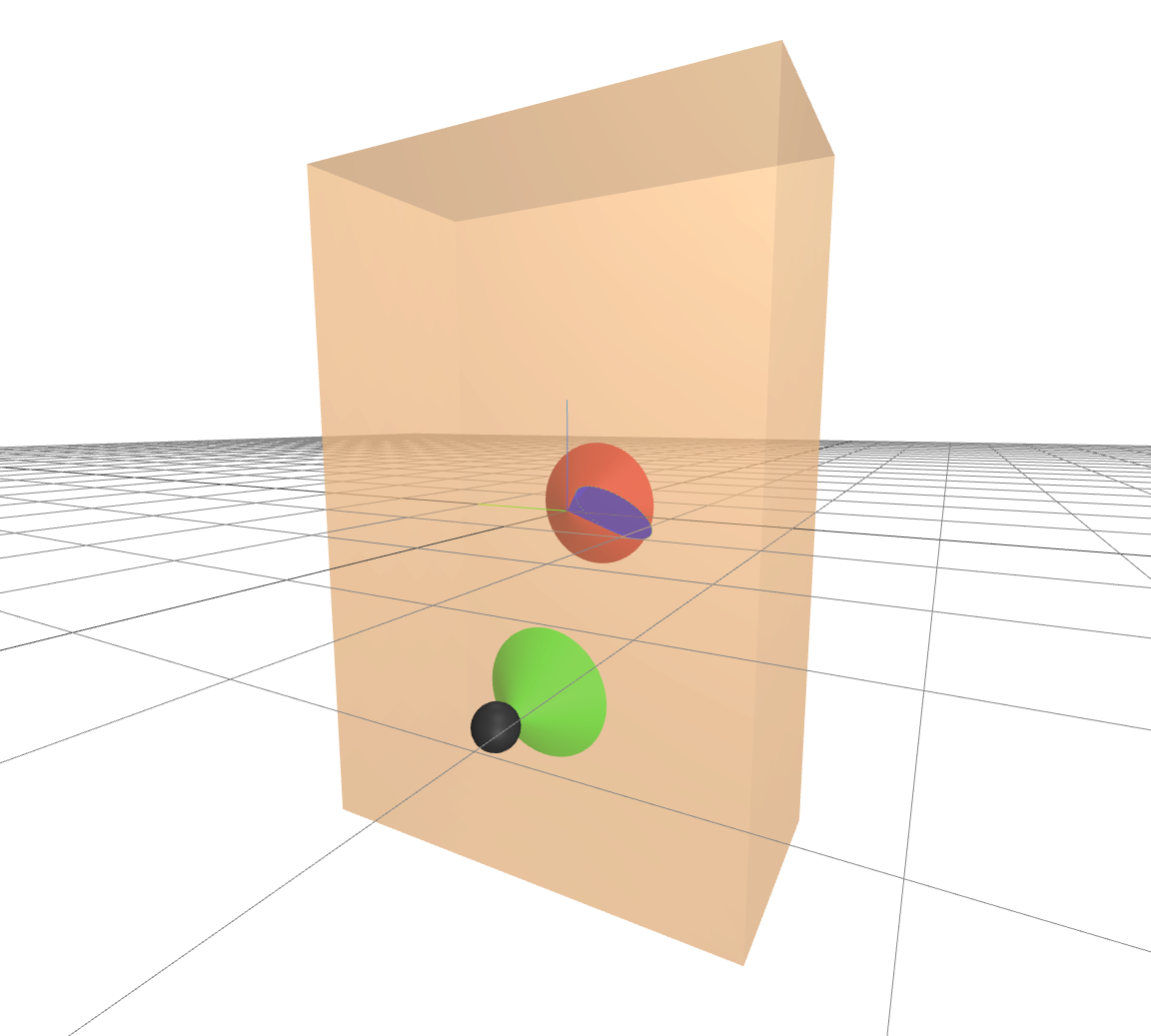
I hope that you immediately notice that the rotational component of
the wrench cone is low dimensional -- due to the cross product, all
vectors in that space must be orthogonal to the vector ${}^Bp^C$. Of
course it's way better to run the notebook yourself and get the 3d
interactive visualization.
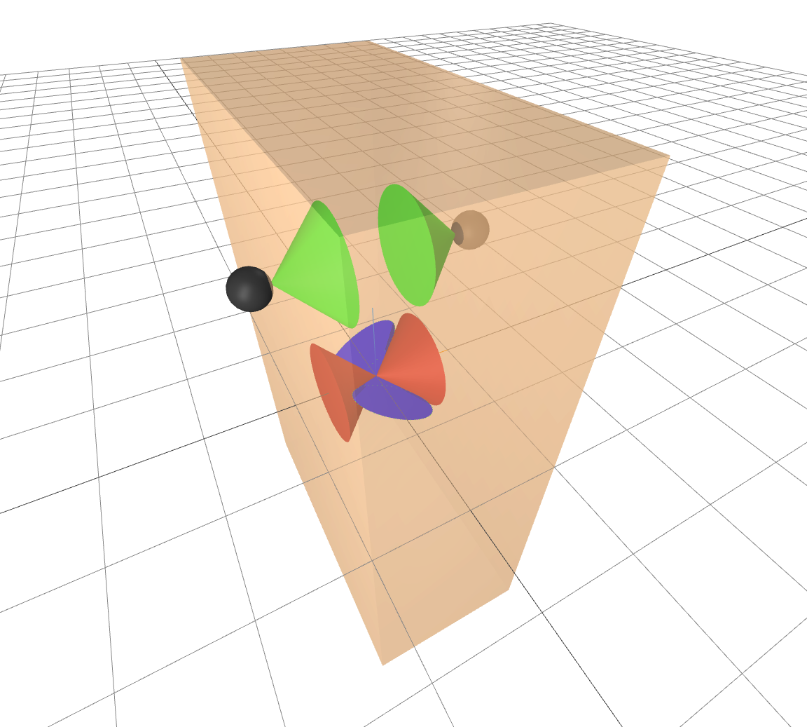
Here is the contact wrench cone for a two contact points on that are
directly opposite from each other:
Notice that while each of the rotational cones are low dimensional,
they span different spaces. Together (as understood by the Minkowski
sum of these two sets) they can resist all pure torques applied at the
body frame. This intuition is largely correct, but this is also where
the projection of the 6d cone onto two 3d cones becomes a bit
misleading. There are some wrenches that cannot be resisted by this
grasp. Specifically, if I were to visualize the wrench cone at the
point directly between the two contact points, we would see that the
wrench cones do not include torques applied directly along the
axis between the two contacts. The two contact points alone, without
torsional friction, are unable to resist torques about that axis.
In practice, the gripper model that we use in our simulation
workflow uses hydroelastic contact, which simulates a contact patch and
can produce torsional friction -- so we can resist moments
around this axis. The exact amount one gets will be proportional to how
hard the gripper is squeezing the object.
Now we can compute the cone of possible wrenches that any set of
contacts can apply on a body -- the contact wrench cone -- by putting all
of the individual contact wrench cones into a common frame and summing
them together. A classic metric for grasping would say that a good grasp
is one where the contact wrench cone is large (can resist many
adversarial wrench disturbances). If the contact wrench cone is all of
$\Re^6$, then we say the contacts have a achieved force
closurePrattichizzo08.
It's worth mentioning that the elegant (linear) spatial algebra of the wrench cones also makes these quantities very suitable for use in optimization (e.g. Dai16).
Colinear antipodal grasps
The beauty of this wrench analysis originally inspires a very
model-based analysis of grasping, where one could try to optimize the
contact locations in order to maximize the contact wrench cone. But our
goals for this chapter are to assume very little about the object that we
are grasping, so we'll (for now) avoid optimizing over the surface of an
object model for the best grasp location. Nevertheless, our model-based
grasp analysis gives us a few very good heuristics for grasping even
unknown objects.
In particular, a good heuristic for a two fingered gripper to have a
large contact wrench cone is to find colinear "antipodal" grasp points.
Antipodal here means that the normal vectors of the contact (the $z$ axis
of the contact frames) are pointing in exactly opposite directions. And
"colinear" means that they are on the same line -- the line between the
two contact points. As you can see in the two-fingered contact wrench
visualization above, this is a reasonably strong heuristic for having a
large total contact wrench cone. As we will see next, we can apply this
heuristic even without knowing much of anything about the objects.
Alternative grasp metrics...
Grasp selection from point clouds
Rather than looking into the bin of objects, trying to recognize
specific objects and estimate their pose, let's consider an approach where
we simply look for graspable areas directly on the (unsegmented) point
cloud. These very geometric approaches to grasp selection can work very
well in practice, and can also be used in simulation to train a
deep-learning-based grasp selection system that can work very well in the
real world and even deal with partial views and occlusions
tenPas17+Mahler17+Zeng18.
Point cloud pre-processing
To get a good view into the bin, we're going to set up multiple RGB-D
cameras. I've used three per bin in all of my examples here. And those
cameras don't only see the objects in the bin; they also see the bins, the
other cameras, and anything else in the viewable workspace. So we have a
little work to do to merge the point clouds from multiple cameras into a
single point cloud that only includes the area of interest.
First, we can crop the point cloud to discard any points that
are from outside the area of interest (which we'll define as an
axis-aligned bounding box immediately above the known location of the
bin).
As we will discuss in some detail below, many of our grasp selection
strategies will benefit from estimating the "normals" of the point
cloud (a unit vector that estimates the normal direction relative to the
surface of the underlying geometry). It is actually better to estimate
the normals on the individual point clouds, making use of the camera
location that generated those points, than to estimate the normal after
the point cloud has been merged.
For sensors mounted on the real world, merging point clouds
requires high-quality camera calibration and must deal with the messy
depth returns. All of the tools from the last chapter are relevant, as
the tasks of merging the point clouds is another instance of the
point-cloud-registration problem. For the perfect depth measurements we
can get out of simulation, given known camera locations, we can skip this
step and simply concatenate the list of points in the point clouds
together.
Finally, the resulting raw point clouds likely include many more points
then we actually need for our grasp planning. One of the standard
approaches for down-sampling the point clouds is using a voxel grid -- regularly
sized cubes tiled in 3D. We then summarize the original point cloud with
exactly one point per voxel (see, for instance Open3D's
note on voxelization). Since point clouds typically only occupy a
small percentage of the voxels in 3D space, we use sparse data structures
to store the voxel grid. In noisy point clouds, this voxelization step is
also a useful form of filtering.
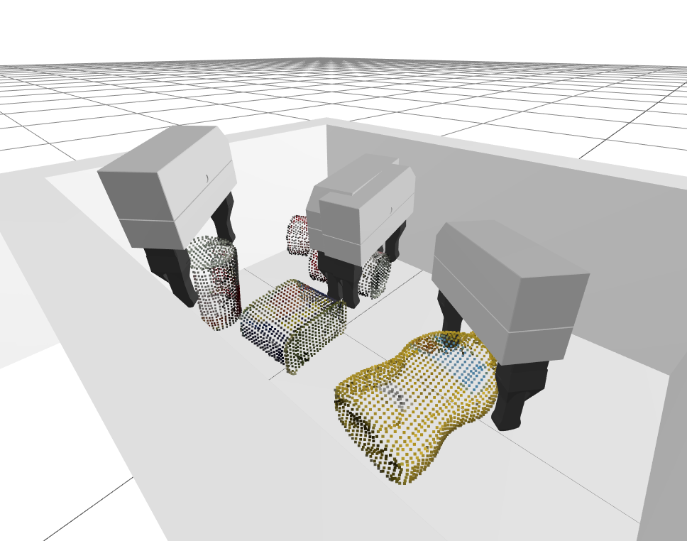
Mustard bottle point clouds
I've produced a scene with three cameras looking at our favorite YCB
mustard bottle. I've taken the individual point clouds (already
converted to the world frame by the
DepthImageToPointCloud system), cropped the point clouds
(to get rid of the geometry from the other cameras), estimated their
normals, merged the point clouds, then down-sampled the point clouds.
The order is important!
I've pushed all of the point clouds to meshcat, but with many of them
set to not be visible by default. Use the drop-down menu to turn them
on and off, and make sure you understand basically what is happening on
each of the steps. For this one, I can also give you the meshcat output
directly, if you don't want to run the code.
Estimating normals and local curvature
The grasp selection strategy that we will develop below will be based on the local geometry (normal direction and curvature) of the scene. Understanding how to estimate those quantities from point clouds is an excellent exercise in point cloud processing, and is representative of other similar point cloud algorithms.
Let's think about the problem of fitting a plane, in a least-squares
sense, to a set of pointsShakarji98. We can describe a plane
in 3D with a position $p$ and a unit length normal vector, $n$. The
distance between a point $p^i$ and a plane is simply given by the
magnitude of the inner product, $\left| (p^i - p)^T n \right|.$ So our
least-squares optimization becomes $$\min_{p, n} \quad \sum_{i=1}^N
\left| (p^i - p)^T n \right|^2, \quad \subjto \quad |n| = 1. $$ Taking
the gradient of the Lagrangian with respect to $p$ and setting it equal
to zero gives us that $$p^* = \frac{1}{N} \sum_{i=1}^N p^i.$$ Inserting
this back into the objective, we can write the problem as $$\min_n n^T W
n, \quad \subjto \quad |n|=1, \quad \text{where } W = \left[ \sum_i (p^i
- p^*) (p^i - p^*)^T \right].$$ Geometrically, this objective is a
quadratic bowl centered at the origin, with a unit circle constraint. So
the optimal solution is given by the (unit-length) eigenvector
corresponding to the smallest eigenvalue of the data matrix, $W$.
And for any optimal $n$, the "flipped" normal $-n$ is also optimal. We
can pick arbitrarily for now, and then flip the normals in a
post-processing step (to make sure that the normals all point towards the
camera origin).
What is really interesting is that the second and third
eigenvalues/eigenvectors also tell us something about the local geometry.
Because $W$ is symmetric, it has orthogonal eigenvectors, and these
eigenvectors form a (local) basis for the point cloud. The smallest
eigenvalue pointed along the normal, and the largest eigenvalue
corresponds to the direction of least curvature (the squared dot product
with this vector is the largest). This information can be very useful for
finding and planning grasps. tenPas17 and others before them
use this as a primary heuristic in generating candidate grasps.
In order to approximate the local curvature of a mesh represented by a
point cloud, we can use our fast nearest neighbor queries to find a
handful of local points, and use this plane fitting algorithm on just
those points. When doing normal estimation directly on a depth image,
people often forgo the nearest-neighbor query entirely; simply using the
approximation that neighboring points in pixel coordinates are often
nearest neighbors in the point cloud. We can repeat that entire
procedure for every point in the point cloud.
I remember when working with point clouds started to become a bigger
part of my life, I thought that surely doing anything moderately
computational like this on every point in some dense point cloud would be
incompatible with online perception. But I was wrong! Even years ago,
operations like this one were often used inside real-time perception
loops. (And they pale in comparison to the number of FLOPs we spend these days
evaluating large neural networks).
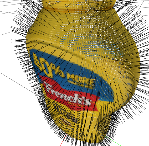
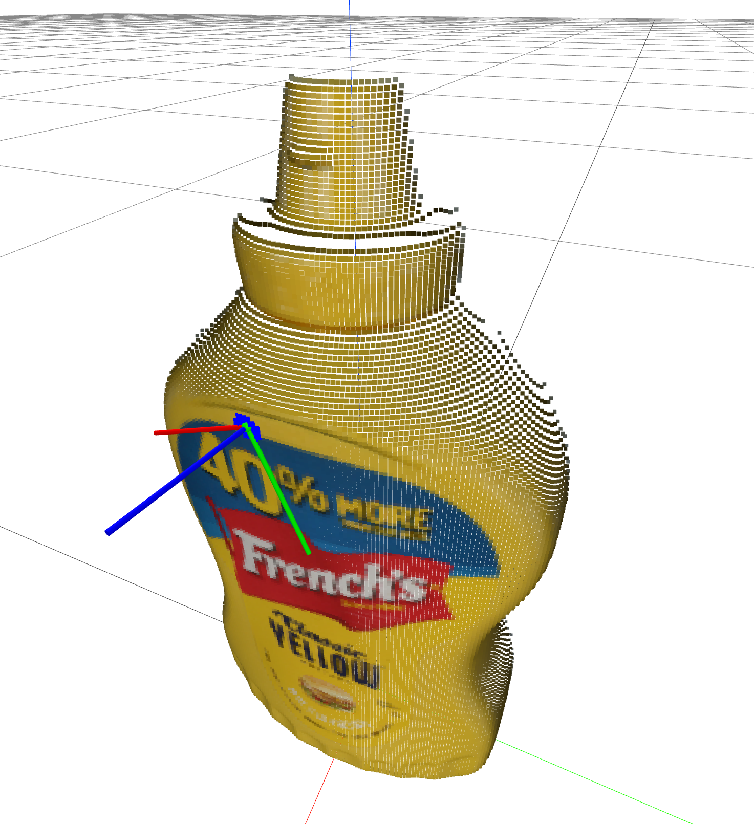
Normals and local curvature of the mustard bottle.
I've coded up the basic least-squares surface estimation algorithm,
with the query point in green, the nearest neighbors in blue, and the
local least squares estimation drawn with our RGB$\Leftrightarrow$XYZ
frame graphic. You should definitely slide it around and see if you can
understand how the axes line up with the normal and local curvature.
You might wonder where you can read more about algorithms of this type.
I don't have a great reference for you. But Radu Rusu was the main author
of the point cloud libraryRusu11, and his thesis has a lot of
nice summaries of the point cloud algorithms of
2010Rusu10.
Evaluating a candidate grasp
Now that we have processed our point cloud, we have everything we need
to start planning grasps. I'm going to break that discussion down into
two steps. In this section we'll come up with a cost function that scores
grasp candidates. In the following section, we'll discuss some very
simple ideas for trying to find grasps candidates that have a low
cost.
Following our discussion of "model-based" grasp selection above, once we pick
up an object -- or whatever happens to be between our fingers when we squeeze --
then we will expect the contact forces between our fingers to have to resist at
least the gravitational wrench (the spatial force due to gravity) of the
object. The closing force provided by our gripper is in the gripper's $x$-axis,
but if we want to be able to pick up the object without it slipping from our
hands, then we need forces inside the friction cones of our contacts to be able to
resist the gravitational wrench. Since we don't know what that wrench will be
(and are somewhat constrained by the geometry of our fingers), a reasonable
strategy is to look at the colinear antipodal points on the surface of the point
cloud which also align with $x$-axis of the gripper. In a real point cloud, we are
unlikely to find perfect antipodal pairs, but finding areas with normals pointing
in nearly opposite directions is a good strategy for grasping!
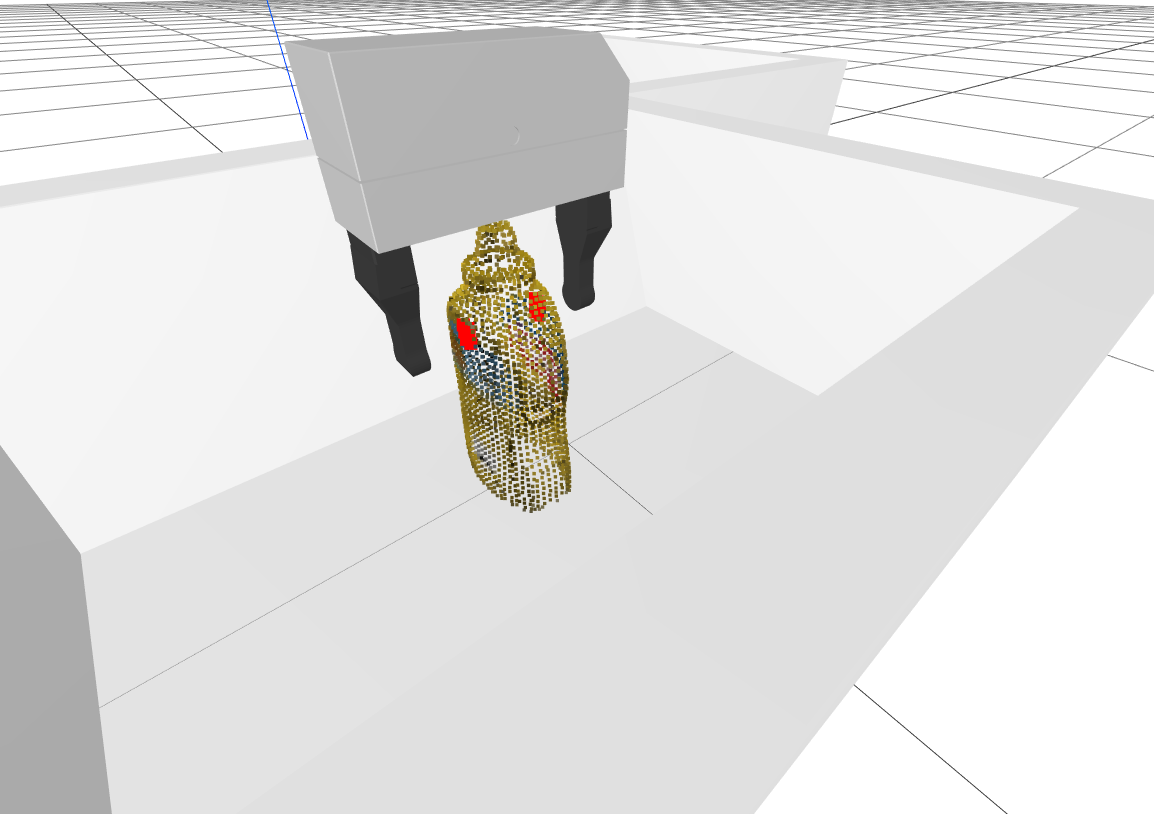
Scoring grasp candidates
In practice, the contact between our fingers and the object(s) will
be better described by a patch contact than by a point contact
(due to the deflection of the rubber fingertips and any deflection of
the objects being picked). So it makes sense to look for patches of
points with agreeable normals. There are many ways one could write
this, I've done it here by transforming the processed point cloud of
the scene into the candidate frame of the gripper, and cropped away all
of the points except the ones that are inside a bounding box between
the finger tips (I've marked them in red in MeshCat). The first term
in my grasping cost function is just reward for all of the points in
the point cloud, based on how aligned their normal is to the $x$-axis
of the gripper: $$\text{cost} = -\sum_i (n^i_{G_x})^2,$$ where
$n^i_{G_x}$ is the $x$ component of the $i$th point in the cropped
point cloud expressed in the gripper frame.
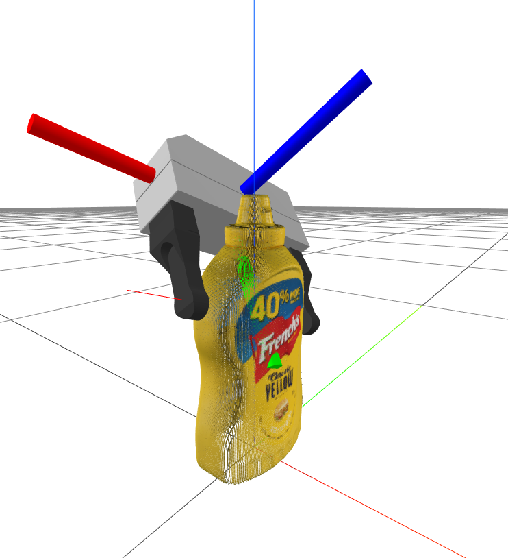
There are other considerations for what might make a good grasp, too.
For our kinematically limited robot reaching into a bin, we might favor
grasps that put the hand in favorable orientation for the arm. In the
grasp metric I've implemented in the code, I added a cost for the hand
deviating from vertical. I can reward the dot product of the vector
world $-z$ vector, $[0, 0, -1]$ with the $y$-axis in gripper frame
rotated into world frame with : $$\text{cost} \mathrel{{+}{=}} -\alpha
\begin{bmatrix} 0 & 0 &-1\end{bmatrix}R^G \begin{bmatrix}0 \\ 1 \\
0\end{bmatrix} = \alpha R^G_{3,2},$$ where $\alpha$ is relative cost
weight, and $R^G_{3,2}$ is the scalar element of the rotation matrix in
the third row and second column.
Finally, we need to consider collisions between the candidate grasp
and both the bins and with the point cloud. I simply return infinite
cost when the gripper is in collision. I've implemented all of those
terms in the notebook, and given you a sliders to move the hand around
and see how the cost changes.
Generating grasp candidates
We've defined a cost function that, given a point cloud from the scene
and a model of the environment (e.g. the location of the bins), can score
a candidate grasp pose, $X^G$. So now we would like to solve the
optimization problem: find $X^G$ that minimizes the cost subject to the
collision constraints.
Unfortunately, this is an extremely difficult optimization problem,
with a highly nonconvex objective and constraints. Moreover, the cost
terms corresponding to the antipodal points is zero for most $X^G$ --
since most random $X^G$ will not have any points between the fingers. As
a result, instead of using the typical mathematical programming solvers,
most approaches in the literature resort to a randomized sampling-based
algorithm. And we do have strong heuristics for picking reasonable
samples.
One heuristic, used for instance in tenPas17, is to use
the local curvature of the point cloud to propose grasp candidates that
have the point cloud normals pointing into the palm, and orients the hand
so that the fingers are aligned with the direction of maximum curvature.
One can move the hand in the direction of the normal until the fingers are
out of collision, and even sample nearby points. We have written an exercise for you to explore this heuristic. But for
our YCB objects, I'm not sure it's the best heuristic; we have a lot of
boxes, and boxes don't have a lot of information to give in their local
curvature.
Another heuristic is to find antipodal point pairs in the point cloud,
and then sample grasp candidates that would align the fingers with those
antipodal pairs. Many 3D geometry libraries support "ray casting"
operations at least for a voxel representation of a point cloud; so a
reasonable approach to finding antipodal pairs is to simply choose a point
at random in the point cloud, then ray cast into the point cloud in the
opposite direction of the normal. If the normal of the voxel found by ray
casting is sufficiently antipodal, and if the distance to that voxel is
smaller than the gripper width, then we've found a reasonable antipodal
point pair.
Generating grasp candidates
As an alternative to ray casting, I've implemented an even simpler
heuristic in my code example: I simply choose a point at random, and
start sampling grasps in orientation (starting from vertical) that
align the $x$-axis of the gripper with the normal of that point. Then
I mostly just rely on the antipodal term in my scoring function to
allow me to find good grasps.
I do implement one more heuristic -- once I've found the points in
the point cloud that are between the finger tips, then I move the hand
out along the gripper $x$-axis so that those points are centered in the
gripper frame. This helps prevent us knocking over objects as we close
our hands to grasp them.
But that's it! It's a very simple strategy. I sample a handful of
candidate grasps and just draw the top few with the lowest cost. If you
run it a bunch of times, I think you will find it's actually quite
reasonable. Every time it runs, it is simulating the objects falling
from the sky; the actual grasp evaluation is actually quite fast.
The corner cases
If you play around with the grasp scoring I've implemented above a little
bit, you will find deficiencies. Some of them are addressed easily (albeit
heuristically) by adding a few more terms to the cost. For instance, I
didn't check collisions of the pre-grasp configuration, but this could be
added easily.
There are other cases where grasping alone is not sufficient as a
strategy. Imagine that you place an object right in one of the corners of
the bin. It might not be possible to get the hand around both sides of the
object without being in collision with either the object or the side. The
strategy above will never choose to try to grab the very corner of a box
(because it always tried to align the sample point normal with the gripper
$x$), and it's not clear that it should. This is probably especially true
for our relatively large gripper. In the setup we used at TRI, we
implemented an additional simple "pushing" heuristic that would be used if
there were point clouds in the sink, but no viable grasp candidate could be
found. Instead of grasping, we would drive the hand down and nudge that
part of the point cloud towards the middle of the bin. This can actually
help a lot!
There are other deficiencies to our simple approach that would be very
hard to address with a purely geometric approach. Most of them come down to
the fact that our system so far has no notion of "objects". For instance,
it's not uncommon to see this strategy result in "double picks" if two
objects are close together in the bin. For heavy objects, it might be
important to pick up the object close to the center of mass, to improve our
chances of resisting the gravitational wrench while staying in our friction
cones. But our strategy here might pick up a heavy hammer by squeezing just
the very far end of the handle.
Interestingly, I don't think the problem is necessarily that the point
cloud information is insufficient, even without the color information. I
could show you similar point clouds and you wouldn't make the same mistake.
These are the types of examples where learning a grasp metric could
potentially help. We don't need to achieve artificial general intelligence
to solve this one; just experience knowing that when we tried to grasp in
someplace before we failed would be enough to improve our grasp heuristics
significantly.
render some point clouds that a human can distinguish but out algorithm would not.
Programming the Task Level
Most of us are used to writing code in a procedural
programming
paradigm; code executes from the top of the program through function calls, branchs
(like if/then statements), for/while loops, etc. It's tempting to try to write our
high-level robot programs like that, too. For the clutter task, I could write
"while there is an object to pick up in the first bin, pick it up and move it to the
second bin; ...". And that is certainly not wrong! But to be a component in a
robotics framework, this high-level program must somehow communicate with the rest
of the system at runtime, including having interfaces to the low-level controllers
that are running at some regular frequency (say 100Hz or even 1kHz). So how do we
author the high-level behaviors (often called "task level") in a way that integrates
seamlessly with the high-rate low-level controls?
There are a few important programming paradigms for authoring the
task-level behavior. Broadly speaking, I would categorize them into three
bins:
Procedural code (in a separate thread) passes messages/events to a
module that lives in the main robot/simulation thread. This is
relatively common in a multi-process message-passing ecosystem like
ROS.
Task-level "policies" can be authored directly as e.g. finite state
machines (FSMs) or "behavior trees", which get evaluated directly in
the robot/simulation loop.
Task-level "planners" can take rules for how task-level behaviors
can be chained together to achieve long-term goals:
In the simplest case, the planner outputs a plan that can be
executed during the robot/simulation loop, just like the trajectories
we've used to plan the motion of the gripper.
If the planner can be run online (e.g. constantly
adjusting/replanning given new sensor information), then it can be
used directly in the robot/simulation loop.
Alternatively, a few planners can actually "compile" their plans
directly into a policy (e.g. in the form of an FSM). Here
is one of the classic examples.
Each of these paradigms has its place, and some researchers heavily favor
one over the other. I'll always remember Rod Brooks writing papers like
Elephants Don't Play Chess to argue against task-level
planningBrooks90+Brooks91+Brooks91a. Rod's "subsumption
architecture" was distinctly in the "task-level policies" category and can
be seen as a precursor to Behavior Trees; it established its credibility by
having success on the early Roomba vacuum cleaners. The planning community
might counter that for truly complicated tasks, it would be impossible for
human programmers to author a policy for all possible permutations /
situations that an AI system might encounter; that planning is the approach
that truly scales. They have addressed some of the initial criticisms about
symbol grounding and modeling requirements with extensions like planning in
belief space and task-and-motion planning, which we will cover in later
parts of the notes.
State Machines and Behavior Trees
Task planning
Task-level planners are based primarily on search. There is a long
history of AI planning as search. STRIPS Fikes71 was perhaps
the earliest, and most famous representation (and algorithm) for
describing planning problems using an initial state, a goal state, and a
set of actions with pre-conditions and effects. Temporal logic (e.g.
linear temporal logic (LTL), metric temporal logic (MTL), signal temporal
logic (STL)) enables the specification to include complex goals or
constraints that evolve over time, such as "event A should eventually
happen after event B". The planning domain definition language (PDDL)
Aeronautiques98+Haslum19 extended the STRIPS representation
to include more expressive features such as typed variables, conditional
effects, and (even temporal logic) quantifiers, and served as the
specification language for a long-running and highly influential series
of ICAPS
planning competitions. These planning competitions gave rise to a
number of highly effective planning algorithms such as GraphPlan
Blum97, HSP Bonet01, Fast-Forward
Hoffmann01, and FastDownward Helmert06. These
planners demonstrated the power of "heurstic search", and strongly
leverage the object-oriented nature of the specification to use
factorization as a strong heuristic.
Large Language Models
In late 2022, of course, a new approach to task "planning" exploded
onto the scene with the rise of large language models (LLMs). It quickly
became clear that the most powerful language models like GPT4 are capable
of producing highly nontrivial plans from very limited natural language
specifications. Careful prompting can be used to guide the LLM to produce
actions that the robot is is able to perform, and it seems that LLMs are
particularly good at writing python code. Using Python, it's even
possible to prompt the LLM to generate a policy rather
than just a plan Liang23. At the time of this writing, their
is still a challenge in automating a depiction of the current environment
as perceived from the robot cameras/sensors into a natural language
prompt, but it seems that this is only a matter of time. Word is that the
rolling release of GPT-4V(ision)
works amazingly well in this capacity.
An informal consensus is that language models make simple planning
problems extraordinarily easy. Importantly, while a search-based planner
might exploit missing requirements / constraints in your specification,
the LLMs output very reasonable plans, using "common sense" to fill in
the gaps. There are still limits to what today's LLMs can achieve in the
way of long-horizon task planning with multi-step reasoning, but clever
prompt engineering can lead to impressive results Yao23.
example?
A simple state machine for "clutter clearing"
For the purposes of clutter clearing in the systems framework, taking
the second approach: writing the task-level behavior "policy" as a simple
state machine will work nicely.
A simple state machine for "clutter clearing"
Show minimal LeafSystem that implements it.
Putting it all together
First, we bundle up our grasp-selection algorithm into a system that
reads the point clouds from 3 cameras, does the point cloud processing
(including normal estimation), and the random sampling, and puts the grasp
selection onto the output port:
Note that we will instantiate this system twice -- once for the bin
located on the positive X axis and again for the system on the negative y
axis. Thanks to the "pull-architecture" in Drake's systems framework, this
relatively expensive sampling procedure only gets called when the
downstream system evaluates the output port.
The work-horse system in this example is the Planner system
which implements the basic state machine, calls the planning functions,
stores the resulting plans in its Context, and evaluates the
plans on the output port:
This system needs enough input / output ports to get the relevant
information into the planner, and to command the downstream
controllers.
Clutter clearing (complete demo)
Maybe add a section here about monte-carlo testing?
Exercises
Assessing static equilibrium
For this problem, we'll use the Coulomb friction model, where $|f_t|
\le \mu f_n$. In other words, the friction force is large enough to
resist any movement up until the force required would exceed $\mu f_n$,
in which case $|f_t| = \mu f_n$.
Consider a box with mass $m$ sitting on a ramp at angle
$\theta$, with coefficient of box $\mu$ in between the sphere and
the ramp:
For a given angle $\theta$, what is the minimum coefficient of
friction required for the box to not slip down the plane? Use $g$
for acceleration due to gravity.
Now consider a flat ground plane with three solid (uniform density)
spheres sitting on it, with radius $r$ and mass $m$. Assume they have
the same coefficient of friction $\mu$ between each other as with the
ground.
For each of the following configurations: could the spheres be in
static equilibrium for some $\mu\in[0,1]$, $m > 0$, $r > 0$? Explain
why or why not. Remember that both torques and forces need to be
balanced for all bodies to be in equilibrium.
To help you solve these problems, we have
to help you build intuition and test your answers. It lets you specify
the configuration of the spheres and then uses the StaticEquilbriumProblem
class to solve for static equilibrium. Use this notebook to help
visualize and think about the system, but for each of the
configurations, you should have a physical explanation for your answer.
(An example of such a physical explanation would be a free body diagram
of the forces and torques on each sphere, and equations for how they
can or cannot sum to zero. This is essentially what
StaticEquilbriumProblem checks for.)
Spheres stacked on top of each other:
One sphere on top of another, offset:
Spheres stacked in a pyramid:
Spheres stacked in a pyramid, but with a distance $d$ in between
the bottom two:
Finally, a few conceptual questions on the
StaticEquilbriumProblem:
Why does it matter what initial guess we specify for the
system? (Hint: what type of optimization problem is this?)
Take a look at the Drake documentation for StaticEquilbriumProblem.
It lists the constraints that are used when it solves for
equilibrium. Which two of these can a free body diagram
answer?
Normal Estimation from Depth
For this exercise, you will investigate a slightly different approach to normal vector estimation. In particular, we can exploit the spatial structure that is already in a depth image to avoid computing nearest neighbors. You will work exclusively in . You will be asked to complete the following steps:
Analyze mathematically how the data matrix constructed from close
clusters of points in a depth image can be used to compute surface normals.
Implement a method to estimate normal vectors from a depth image,
without computing nearest neighbors.
Reason about a scenario where the depth image-based solution will
not be as performant as computing nearest-neighbors.
Analytic Antipodal Grasping
So far, we have used sampling-based methods to find antipodal grasps - but can we have find one analytically if we knew the equation of the object shape? For this exercise, you will analyze and implement a correct-by-construction method to find antipodal points using symbolic differentiation and MathematicalProgram. You will work exclusively in . You will be asked to complete the following steps:
Prove that antipodal points are critical points of an energy
function defined on the shape.
Prove the converse does not hold.
Implement a method to find these antipodal points using
MathematicalProgram.
Analyze the Hessian of the energy function and its relation to the
type of antipodal grasps.
Grasp Candidate Generation
In the chapter notebook, we generated grasp candidates using the
antipodal heuristic. In this exercise, we will investigate an
alternative method for generating grasp candidates based on local
curvature, similar to the one proposed in tenPas17. This
exercise is implementation-heavy, and you will work exclusively in .
Behavior Trees
Let's reintroduce the terminology of behavior trees. Behavior trees
provide a structure for switching between different tasks in a way that
is both modular and reactive. Behavior trees are a directed rooted tree
where the internal nodes manage the control flow and the leaf nodes are
actions to be executed or conditions to be evaluated. For example, an
action may be to "pick ball". This action can succeed or fail. A
condition may be "Is my hand empty?" which can be true (thus the
condition succeeds) or can be false (the condition fails).
More specifically, each node is periodically checked. In turn it will
check its children, and report status as success, failure or running
depending on its childrens' statuses. There are different categories
of control flow nodes, but we'll consider two categories of control
flow nodes:
Sequence Node: ($\rightarrow$)
Sequence nodes execute
each of the child behaviors left to right. The sequence returns failure
if any of the children fail and running if any of the children are
running. One way to think about this operator is that
a sequence node takes an "and" over all of the child behaviors.
Fallback Node: (?)
Fallback nodes also execute each of the
child behaviors one after another. However, fallback succeeds if any
of the children succeed. One way to think about this operator is
that the fallback node takes an "or" over all of the children
behaviors.
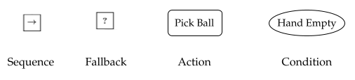
The symbols are visualized below. Sequence nodes are represented as an
arrow in a box, fallback nodes are represented as a question mark in a box,
actions are inside boxes and conditions are inside ovals.
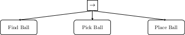
Let's apply our understanding of behavior trees in the context of a
simple task where a robot's goal is to: find a ball, pick the ball up and
place the ball in a bin. We can describe task with the high-level behavior
tree:
Confirm to yourself that this small behavior tree captures the task! We
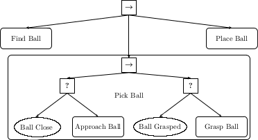
can go one level deeper and expand out our "Pick Ball" behavior:
The pick ball behavior can be considered as such: Let's start with the
left branch. If the ball is already close, the condition "Ball Close?"
returns true. If the ball is not close, we execute an action to "Approach
ball", thus making the ball close. Thus either the ball is already close
(i.e. the condition "Ball Close?" is true) or we approach the ball (i.e.
the action "Approach ball" is successfully executed) to make the ball
close. Given that the ball is now close, we consider the right branch of
the pick action. If the ball is already grasped, the condition "Ball
Grasped?" returns true. if the ball is not grasped, we execute the action,
"Grasp Ball".
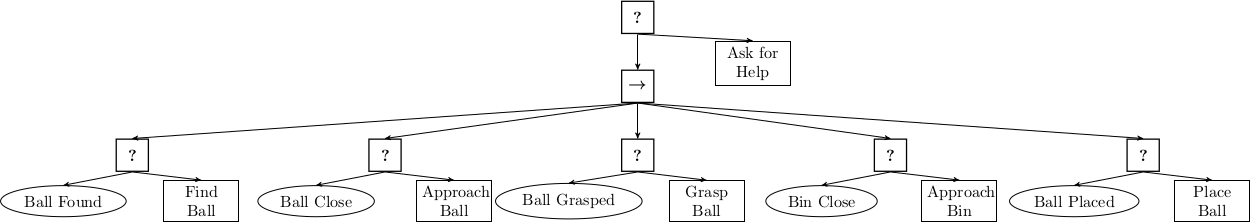
We can expand our our behavior tree even further to give our full
behavior:
Behavior Tree for Pick-Up Task
Here we've added the behavior that if the robot cannot complete the
task, it can ask a kind human for help. Take a few minutes to walk through
the behavior tree and convince yourself it encodes the desired task
behavior.
We claimed behavior trees enable reactive behavior. Let's explore
that. Imagine we have a robot executing our behavior tree. As the robot is executing the
action "Approach Bin", a rude human knocks the ball out of the robot's
hand. The ball rolls to a position that the robot can still see, but is
quite far away. Following the logic of the behavior tree, what
condition fails and what action is executed because of this?
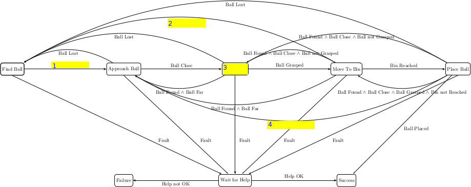
Another way to mathematically model computation is through finite
state machines (FSM). Finite state machines are composed of states,
transitions and events. We can encode the behavior of our behavior tree
for our pick-up task through a finite state machine, as shown below:
We have left a few states and transitions blank. Your task is to fill in
those 4 values such that the finite state machine produces the same
behavior as the behavior tree.
From this simple task we can see that while finite state machines can
often be easy to understand and intuitive, they can quickly get quite
messy!
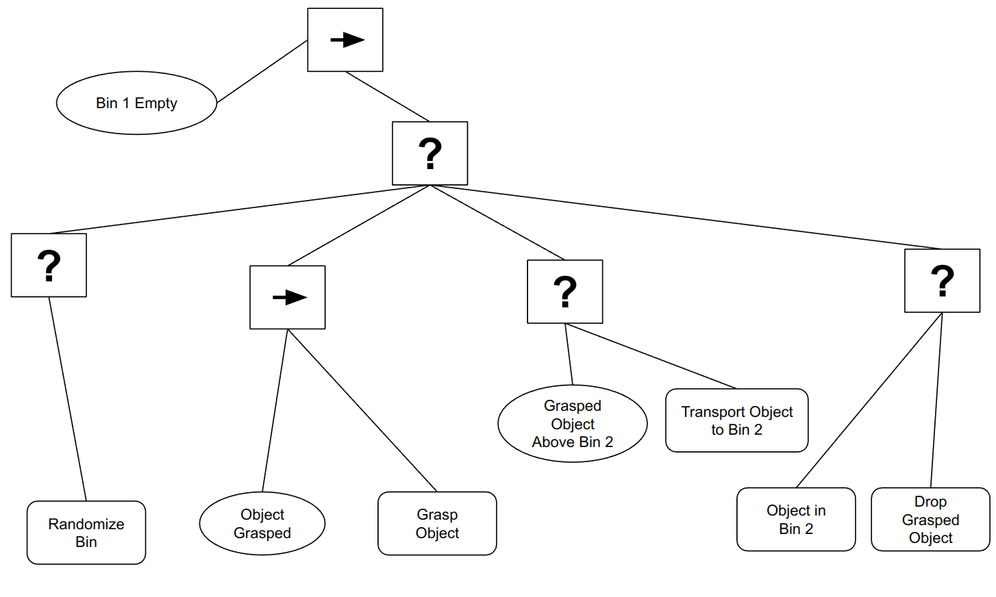
Throughout this chapter and the lectures we've discussed a bin
picking task. Our goal is to now capture the behavior of the
bin-picking task using a behavior tree. We want to encode the following
behavior: while Bin 1 is not empty, we are going to select a feasible
grasp within the bin, execute our grasp and transport what's within our
grasp to Bin 2. If there are still objects within Bin 1, but we cannot
find a feasible grasp, assume we have some action that shakes the bin,
hence randomizing the objects and (hopefully) making feasible grasps
available.
We define the following conditions:
"Bin 1 empty?
"Feasible Grasp Exists?"
"Grasp selected?"
"Grasped Object(s) above Bin 2?"
"Object Grasped?"
"Object(s) in Bin 2?"
And the following actions:
"Drop grasped object(s) into Bin 2"
"Grasp Object(s)"
"Select Grasp"
"Randomize Bin"
"Transport grasped object(s) to above Bin 2"
Using these conditions, actions and our two control flow nodes
(Sequence and Fallback), we want you to draw a behavior tree that
captures the behavior of our bin picking task. To get you started, we
have included a "rough draft" behavior tree below, but it's broken in a
number of places (e.g., some branches might be missing, some control
flow nodes/actions/conditions might have the wrong type, etc.):
Your job is to identify all of the places where it's broken, and draw
your own correct behavior tree with all the broken components fixed.
We claimed behavior trees are modular. Their modularity comes from the
fact that we can write reusable snippets of code that define actions and
conditions and then compose them using behavior trees. For example, we can
imagine that the "Select Grasp" action from part (c) is implemented using
the antipodal grasping mechanism we have built up throughout this chapter.
And the "Transport grasped object(s) to above Bin 2" action could be
implemented using the pick and place tools we developed in Chapter 3.
Source: The scenario and figures for parts (a) and (b) of this exercise
are inspired by material in Colledanchise18
Sampling Antipodal Grasps
For this exercise we will practice sampling antipodal grasps with your own
initials. You will explore how ray casting can be used to find antipodal point pairs,
which form the basis of a grasp. You will work exclusively in
. You will be asked to complete the following
steps:
Sample antipodal point pairs from a mesh.
Filter antipodal point pairs based on grasp heuristics.
Use the grasp heuristics to manipulate custom meshes in a scene.
References
Berk Calli and Arjun Singh and James Bruce and Aaron Walsman and Kurt Konolige and Siddhartha Srinivasa and Pieter Abbeel and Aaron M Dollar,
"Yale-CMU-Berkeley dataset for robotic manipulation research",
The International Journal of Robotics Research, vol. 36, no. 3, pp. 261--268, 2017.
Gregory Izatt and Russ Tedrake,
"Generative Modeling of Environments with Scene Grammars and Variational Inference",
Proceedings of the 2020 IEEE International Conference on Robotics and Automation (ICRA) , 2020.
[ link ]
Ryan Elandt and Evan Drumwright and Michael Sherman and Andy Ruina,
"A pressure field model for fast, robust approximation of net contact force and moment between nominally rigid objects",
, pp. 8238-8245, 11, 2019.
Domenico Prattichizzo and Jeffrey C Trinkle,
"Grasping",
Springer Handbook of Robotics , pp. 671-700, 2008.
Hongkai Dai,
"Robust multi-contact dynamical motion planning using contact wrench set",
PhD thesis, Massachusetts Institute of Technology, 2016.
[ link ]
Andreas ten Pas and Marcus Gualtieri and Kate Saenko and Robert Platt,
"Grasp pose detection in point clouds",
The International Journal of Robotics Research, vol. 36, no. 13-14, pp. 1455--1473, 2017.
Jeffrey Mahler and Jacky Liang and Sherdil Niyaz and Michael Laskey and Richard Doan and Xinyu Liu and Juan Aparicio Ojea and Ken Goldberg,
"Dex-net 2.0: Deep learning to plan robust grasps with synthetic point clouds and analytic grasp metrics",
arXiv preprint arXiv:1703.09312, 2017.
Andy Zeng and Shuran Song and Kuan-Ting Yu and Elliott Donlon and Francois R Hogan and Maria Bauza and Daolin Ma and Orion Taylor and Melody Liu and Eudald Romo and others,
"Robotic pick-and-place of novel objects in clutter with multi-affordance grasping and cross-domain image matching",
2018 IEEE international conference on robotics and automation (ICRA) , pp. 1--8, 2018.
Craig M Shakarji,
"Least-squares fitting algorithms of the NIST algorithm testing system",
Journal of research of the National Institute of Standards and Technology, vol. 103, no. 6, pp. 633, 1998.
Radu Bogdan Rusu and Steve Cousins,
"3D is here: Point Cloud Library (PCL)",
Proceedings of the IEEE International Conference on Robotics and Automation (ICRA) , May 9-13, 2011.
Radu Bogdan Rusu,
"Semantic 3D Object Maps for Everyday Manipulation in Human Living Environments",
PhD thesis, Institut für Informatik der Technischen Universität München, 2010.
R. A. Brooks,
"Elephants Don't Play Chess",
Robotics and Autonomous Systems, vol. 6, pp. 3--15,, 1990.
Rodney A. Brooks,
"Intelligence Without Reason",
, no. 1293, April, 1991.
Rodney A. Brooks,
"Intelligence without representation",
Artificial Intelligence, vol. 47, pp. 139-159, 1991.
Richard E Fikes and Nils J Nilsson,
"STRIPS: A new approach to the application of theorem proving to problem solving",
Artificial intelligence, vol. 2, no. 3-4, pp. 189--208, 1971.
Constructions Aeronautiques and Adele Howe and Craig Knoblock and ISI Drew McDermott and Ashwin Ram and Manuela Veloso and Daniel Weld and David Wilkins SRI and Anthony Barrett and Dave Christianson and others,
"PDDL| the planning domain definition language",
Technical Report, Tech. Rep., 1998.
Patrik Haslum and Nir Lipovetzky and Daniele Magazzeni and Christian Muise and Ronald Brachman and Francesca Rossi and Peter Stone,
"An introduction to the planning domain definition language", Springer
, vol. 13, 2019.
Avrim L Blum and Merrick L Furst,
"Fast planning through planning graph analysis",
Artificial intelligence, vol. 90, no. 1-2, pp. 281--300, 1997.
Blai Bonet and Héctor Geffner,
"Planning as heuristic search",
Artificial Intelligence, vol. 129, no. 1-2, pp. 5--33, 2001.
Jörg Hoffmann,
"FF: The fast-forward planning system",
AI magazine, vol. 22, no. 3, pp. 57--57, 2001.
Malte Helmert,
"The fast downward planning system",
Journal of Artificial Intelligence Research, vol. 26, pp. 191--246, 2006.
Jacky Liang and Wenlong Huang and Fei Xia and Peng Xu and Karol Hausman and Brian Ichter and Pete Florence and Andy Zeng,
"Code as policies: Language model programs for embodied control",
2023 IEEE International Conference on Robotics and Automation (ICRA) , pp. 9493--9500, 2023.
Shunyu Yao and Dian Yu and Jeffrey Zhao and Izhak Shafran and Thomas L Griffiths and Yuan Cao and Karthik Narasimhan,
"Tree of thoughts: Deliberate problem solving with large language models",
arXiv preprint arXiv:2305.10601, 2023.
Michele Colledanchise and Petter Ogren,
"Behavior trees in robotics and AI: An introduction", CRC Press
, 2018.