In the last chapter, we developed an initial solution to moving objects
around, but we made one major assumption that would prevent us from using it
on a real robot: we assumed that we knew the initial pose of the object. This
chapter is going to be our first pass at removing that assumption, by
developing tools to estimate that pose using the information obtained from the
robot's depth cameras. The tools we develop here will be most useful when you
are trying to manipulate known objects (e.g. you have a mesh file of
their geometry) and are in a relatively uncluttered environment. But
they will also form a baseline for the more sophisticated methods we will
study.
The approach that we'll take in this chapter is based on geometry. Not all
perception systems these days use geometry explicitly; many deep learning
approaches learn more direct maps from pixels. But many deep learning
approaches do build heavily on geometry, and indeed the last few years
have also brought a revolution in geometry processing (dense reconstruction,
text to 3D, etc.). Some of this was fueled initially by applications in
autonomous driving and virtual/augmented reality in addition to manipulation,
which brought advanced sensors and fantastic new algorithms.
So we will start with geometry because it can provide a solid foundation
for our explorations in perception. I must state one caveat -- we will use
"pose estimation" as our goal for this chapter because it is concrete and
immediately useful. But I would say that I try not to use explicit
pose estimation as a concept in our most advanced manipulation systems; in
addition to assuming known objects, accurately estimating the pose of an
object can be difficult (due to partial views and/or occlusions) and it is
often more than we actually need to achieve our manipulation goals.
Cameras and depth sensors
Just as we had many choices when selecting the robot arm and hand, we
have many choices for instrumenting our robot/environment with sensors. Even
more so than our robot arms, the last few years have seen incredible
improvements in the quality and reductions in cost and size for these
sensors. This is largely thanks to the cell phone industry, but the race
for autonomous cars has been fueling high-end sensors as well.
These changes in hardware quality have caused sometimes dramatic changes
in our algorithmic approaches. For example, estimation can be much easier
when the resolution and frame rate of our sensors is high enough that not
much can change in the world between two images; this undoubtedly
contributed to the revolutions in the field of "simultaneous localization
and mapping" (SLAM) we have seen over the last decade or so.
One might think that the most important sensors for manipulation are the
touch sensors (you might even be right!). But in practice today, most of
the emphasis is on camera-based and/or range sensing. At very least, we
should consider this first, since our touch sensors won't do us much good if
we don't know where in the world we need to touch.
Traditional cameras, which we think of as a sensor that outputs a color
image at some framerate, play an important role. But robotics makes heavy
use of sensors that make an explicit measurement of the distance (between
the camera and the world) or depth; sometimes in addition to color and
sometimes in lieu of color.
Depth sensors
Primarily RGB-D (ToF vs projected texture stereo vs ...) cameras and Lidar
The cameras we are using in this course are Intel RealSense D415.
Monocular depth.
Learned stereo Shankar22.
How the kinect works in 2 minutes: https://www.youtube.com/watch?v=uq9SEJxZiUg
Simulation
There are a number of levels of fidelity at which one can simulate a
camera like the D415. We'll start our discussion here using an "ideal"
RGB-D camera simulation -- the pixels returned in the depth image
represent the true geometric depth in the direction of each pixel
coordinate. In that is represented by the
RgbdSensor system, which can be wired up directly to the
SceneGraph.
The signals and systems abstraction here is encapsulating a lot of
complexity. Inside the implementation of that system is a complete
rendering engine, like one that you will find in high-end computer games.
Drake actually supports multiple rendering
engines; for the purposes of this class we will primarily use an
OpenGL-based renderer (built on VTK) that
is suitable for real-time simulation. Drake can also connect to high-end
physically-based
rendering (PBR) engines which use ray tracing, such as the Cycles renderer
provided by Blender (see the Drake-Blender
project). These are potentially useful for rendering higher quality
images e.g. to train a deep perception system or make a beautiful
presentation.
Simulating an RGB-D camera
As a simple example of depth cameras in drake, I've constructed a
scene with a single object (the mustard bottle from the YCB
dataset), and added an RgbdSensor to the diagram. Once
this is wired up, we can simply evaluate the output ports in order to
obtain the color and depth images:
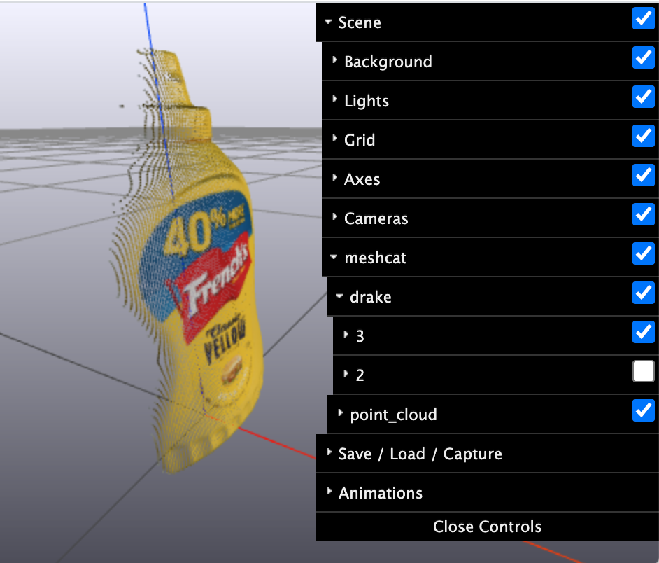
Please make sure you spend a minute
with the MeshCat visualization (available
here). You'll see a camera and the camera frame, and you'll see the
mustard bottle as always... but it might look a little funny. That's
because I'm displaying both the ground truth mustard bottle model
and the point cloud rendered from the cameras. You can use the
MeshCat GUI to uncheck the ground truth visualization (image right), and you'll be able to see just the point cloud.
Remember that, in addition to looking at the source code if you like,
you can always inspect the block diagram to understand what is happening
at the "systems level". Here is the diagram used in this example.
In the HardwareStation workflow, if cameras are declared
in the scenario data (e.g. Yaml description), then the
RgbdSensors are added automatically inside the
HardwareStation diagram, and their output ports exposed as
outputs (in order to match the true interface that we have with the
hardware).
Sensor noise and depth dropouts
Real depth sensors, of course, are far from ideal -- and errors in
depth returns are not simple Gaussian noise, but rather are dependent
on the lighting conditions, the surface normals of the object, and the
visual material properties of the object, among other things. The
color channels are an approximation, too. Even our high-end renderers
can only do well if we add sufficiently accurate geometries, materials
and lighting sources to our scene, and it is very hard to capture all
of the nuances of a real environment. We will examine real sensor
data, and the gaps between modeled sensors and real sensors, after we
start understanding some of the basic operations.
Real depth sensors are
messy. The red pixels in the far right image are missed returns -- the
depth sensor returned "maximum depth". Missed returns, especially on
the edges of objects (or on reflective objects) are a common sighting in
raw depth data. This figure is reproduced from
Sweeney18a.
Occlusions and partial views
The view of the mustard bottle in the example above makes one primary
challenge of working with cameras very clear. Cameras don't get to see
everything! They only get line of sight. If you want to get points from
the back of the mustard bottle, you'll need to move the camera. And if
the mustard bottle is sitting on the table, you'll have to pick it up if
you ever want to see the bottom. This situation gets even worse in
cluttered scenes, where we have our views of the bottle occluded by
other objects. Even when the scene is not cluttered, a head-mounted or
table-mounted camera is often blocked by the robot's hand when it goes to
do manipulation -- the moments when you would like the sensors to be at
their best is often when they give no information!
It is quite common to mount a depth camera on the robot's wrist in
order to help with the partial views. But it doesn't completely resolve
the problem. All of our depth sensors have both a maximum range and a
minimum range. The RealSense D415 returns matches from about 0.3m to
1.5m. That means for the last 30cm of the approach to the object --
again, where we might like our cameras to be at their best -- the object
effectively disappears!
When luxury permits, we try to put as many cameras as we can
into the robot's environment. In this dish-loading testbed at TRI
where we put a total of eight cameras into the scene (it still doesn't
resolve the occlusion problem).
Representations for geometry
There are many different representations for 3D geometry, each of which
can be more or less suitable for different computations. Often we can
convert between these representations; though sometimes that conversion can
be lossy. Examples include triangulated surface meshes and tetrahedral
volumetric meshes, voxel/occupancy grids, and implicit representations of
geometry like the signed distance functions and Neural Radiance Fields
(NeRFs), which have become very popular again recently as representations
in deep learning for 3D visionPark19+Mildenhall21. But the
representations that we will start with here are depth images and
point clouds.
The data returned by a depth camera takes the form of an image, where
each pixel value is a single number that represents the distance between the
camera and the nearest object in the environment along the pixel direction.
If we combine this with the basic information about the camera's intrinsic
parameters (e.g. lens parameters, stored in the CameraInfo
class in Drake) then we can transform this depth image representation into a
collection of 3D points, $s_i$. I use $s$ here because they are commonly referred
to as the "scene points" in the algorithms we will present below. These points are
expressed in some reference frame described by a rigid transform and (optionally) a
color value or other information attached; this is the point cloud
representation. In the DepthImageToPointCloud system in Drake, the
default frame is the camera frame, $^CX^{s_i}$, but the system also accepts $^PX^C$
on a (optional) input port to make it easy to transform them into another frame
(such as the world frame).
As depth sensors have become so pervasive the field has built up
libraries of tools for performing basic geometric operations on point
clouds, and that can be used to transform back and forth between
representations. We implement many of of the basic operations directly in
Drake. There are also open-source tools like the Open3D library that are available if you
need more. Many older projects used the Point Cloud Library (PCL), which is now
defunct but still has some very useful documentation.
It's important to realize that the conversion of a depth image into a
point cloud does lose some information -- specifically the information
about the ray that was cast from the camera to arrive at that point. In
addition to declaring "there is geometry at this point", the depth image
combined with the camera pose also implies that "there is no geometry in the
straight line path between camera and this point". We will make use of this
information in some of our algorithms, so don't discard the depth images
completely! More generally, we will find that each of the different
geometry representations have strengths and weaknesses -- it is very common
to keep multiple representations around and to convert back and forth
between them.
Point cloud registration with known
correspondences
Let us begin to address the primary objective of the chapter -- we have a
known object somewhere in the robot's workspace, we've obtained a point
cloud from our depth cameras. How do we estimate the pose of the object,
$X^O$?
One very natural and well-studied
formulation of this problem comes from the literature on point cloud
registration (also known as point set registration or scan matching).
Given two point clouds, point cloud registration aims to find a rigid
transform that optimally aligns the two point clouds. For our purposes,
that suggests that our "model" for the object should also take the form of a
point cloud (at least for now). We'll describe that object with a list of
model points, $m_i$, with their pose described in the object frame:
$^OX^{m_i}.$
The hypothes.is comment is right, I should add a diagram w/ model and scene points.
Our second point cloud will be the scene points, $s_i$, that we
obtain from our depth camera, transformed (via the camera intrinsics) into
the camera coordinates, $^CX^{s_i}$. I'll use $N_m$ and $N_s$ for the
number of model and scene points, respectively.
Let us assume, for now, that we also know $X^C.$ Is this reasonable? In
the case of a wrist-mounted camera, this would amount to solving the
forward kinematics of the arm. In an environment-mounted camera, this is
about knowing the pose of the cameras in the world. Small errors in
estimating those poses, though, can lead to large artifacts in the
estimated point clouds. We therefore take great care to perform camera
extrinsics calibration; I've linked to our calibration code in the appendix. Note that if you have a mobile
manipulation platform (an arm mounted on a moving base), then all of these
discussions still apply, but you likely will perform all of your
registration in the robot's frame instead of the world frame.
The second major assumption that we will make in this section is
"known correspondences". When I say "correspondence" here, I mean that for
each point in the scene point cloud, we can pair it with a specific
point in the model point cloud; for instance, this might be the case if
each point had a unique color that we could perceive reliably through the
camera. This is not a reasonable assumption in practice, but it
helps us get started. To represent this mapping in our equations, I'll use
a correspondence vector $c \in [1,N_m]^{N_s}$, where $c_i = j$ denotes that
scene point $s_i$ corresponds with model point $m_j$. Note that we do not
assume that these correspondences are one-to-one. Every scene point
corresponds to some model point, but the converse is not true, and multiple
scene points may correspond to the same model point.
As a result, the point-cloud registration problem is simply an (inverse)
kinematics problem. We can write the model points and the scene points in a
common frame (here the world frame), $${}^W p^{m_{c_i}} = {}^W X^O \: {}^Op^{m_{c_i}}
= {}^W X^C \: {}^Cp^{s_i},$$ leaving a single unknown transform, $X^O$, for which
we must solve. In the previous chapter I argued for using differential
kinematics instead of inverse kinematics; why is my story different here?
Differential kinematics can still be useful for perception, for example if
we want to track the pose of an object after we acquire its initial pose.
But unlike the robot case, where we can read the joint sensors to get our
current state, in perception we need to solve this harder problem at least
once.
What does a solution for $X^O$ look like? Each model point gives us
three constraints, when $p^{s_i} \in \Re^3.$ The exact number of unknowns
depends on the particular representation we choose for the pose, but almost
always this problem is dramatically over-constrained. Treating each point
as hard constraints on the relative pose would also be very susceptible to
measurement noise. As a result, it will serve us better to try to find a
pose that describes the data, e.g., in a least-squares sense: $$\min_{X
\in \mathrm{SE}(3)} \sum_{i=1}^{N_s} \| X \: {}^Op^{m_{c_i}} - X^C \:
{}^Cp^{s_i}\|^2.$$ Here I have used the notation $\mathrm{SE}(3)$ for the
"special Euclidean
group," which is the standard notation saying the $X$ must be a valid
rigid transform.
To proceed, let's pick a particular representation for the pose to work
with. I will use 3x3 rotation matrices here; the approach I'll describe
below also has an equivalent in quaternion formHorn87. To
write the optimization above using the coefficients of the rotation matrix
and the translation as decision variables, I have: \begin{align} \min_{p,
R} \quad& \sum_{i=1}^{N_s} \| p + R \: {}^Op^{m_{c_i}} - X^C
\: {}^Cp^{s_i} \|^2, \\ \subjto \quad& R^T = R^{-1}, \quad \det(R) = +1.
\nonumber \end{align} The constraints are needed because not every 3x3
matrix is a valid rotation matrix; satisfying these constraints ensures that
$R$ is a valid rotation matrix. In fact, the constraint $R^T =
R^{-1}$ is almost enough by itself; it implies that $\det(R) = \pm 1.$ But a
matrix that satisfies that constraint with $\det(R) = -1$ is called an "improper
rotation", or a rotation plus a reflection across the axis of
rotation.
Let's think about the type of optimization problem we've formulated so
far. Given our decision to use rotation matrices, the term $p +
R{}^Op^{m_{c_i}} - X^C {^Cp^{s_i}}$ is linear in the decision variables
(think $Ax \approx b$), making the objective a convex quadratic. How about
the constraints? The first constraint is a quadratic equality constraint
(to see it, rewrite it as $RR^T=I$ which gives 9 constraints, each quadratic
in the elements of $R$). The determinant constraint is cubic in the
elements of $R$.
Rotation-only point registration in 2D
I would like you to have a graphical sense for this optimization
problem, but it's hard to plot the objective function with 9+3 decision
variables. To whittle it down to the essentials that I can plot, let's
consider the case where the scene points are known to differ from the
model points by a rotation only (this is famously known as the Wahba
problem). To further simplify, let's consider the problem in 2D
instead of 3D.
In 2D, we can actually linearly parameterize a rotation matrix with
just two variables: $$R = \begin{bmatrix} a & -b \\ b & a\end{bmatrix}.$$
With this parameterization, the constraints $RR^T=I$ and the determinant
constraints are identical; they both require that $a^2 + b^2 = 1.$
The $x$ and $y$ axes of this
plot correspond to the parameters $a$, and $b$, respectively, that define
the 2D rotation matrix, $R$. The green quadratic bowl is the objective
$\sum_i \| R \: {}^O p^{m_{c_i}} - p^{s_i}\|^2,$ and the red open cylinder is
the rotation matrix constraint. Click here for the interactive
version.
Is that what you expected? I generated this plot using just two
model/scene points, but adding more will only change the shape of the
quadratic, but not its minimum. And on the interactive version of the
plot, I've added a slider so that you control the parameter, $\theta$,
that represents the ground truth rotation described by $R$. Try it
out!
In the case with no noise in the measurements (e.g. the scene points
are exactly the model points modified by a rotation matrix), then the
minimum of the objective function already satisfies the constraint. But
if you add just a little noise to the points, then this is no longer
true, and the constraint starts to play an important role.
The geometry should be roughly the same in 3D, though clearly in much
higher dimensions. But I hope that the plot makes it perhaps a little less
surprising that this problem has an elegant numerical solution based on the
singular value decomposition (SVD).
What about translations? There is a super important insight that allows
us to decouple the optimization of rotations from the optimization of
translations. The insight is this: the relative position between
points is affected by rotation, but not by translation. Therefore, if we
write the points relative to some canonical point on the object, we can
solve for rotations alone. Once we have the rotation, then we can back out
the translations easily. For our least squares objective, there is even a
"correct" canonical point to use -- the central point (like the
center of mass if all points have equal mass) under the Euclidean
metric.
Therefore, to obtain the solution to the problem, \begin{align}
\min_{p\in\Re^3,R\in\Re^{3\times3}} \quad & \sum_{i=1}^{N_s} \| p + R
\: {}^Op^{m_{c_i}} - p^{s_i}\|^2, \\ \subjto \quad & RR^T =
I,\end{align} first we define the central model and scene points, $\bar{m}$
and $\bar{s}$, with positions given by $${}^Op^\bar{m} = \frac{1}{N_s}
\sum_{i=1}^{N_s} {}^Op^{m_{c_i}}, \qquad p^\bar{s} = \frac{1}{N_s}
\sum_{i=1}^{N_s} p^{s_i}.$$ If you are curious, these come from taking the
gradient of the Lagrangian
with respect to $p$, and setting it equal to zero: $$\sum_{i=1}^{N_s} 2 (p +
R \: {}^Op^{m_{c_i}} - p^{s_i}) = 0 \Rightarrow p^* = \frac{1}{N_s}
\sum_{i=1}^{N_s} p^{s_i} - R^*\left(\frac{1}{N_s} \sum_{i=1}^{N_s}
{}^Op^{m_{c_i}}\right),$$ but don't forget the geometric interpretation
above. This is just another way to see that we can substitute the
right-hand side in for $p$ in our objective and solve for $R$ by itself.
To find $R$, compose the data matrix $$W = \sum_{i=1}^{N_s} (p^{s_i} -
p^\bar{s}) ({}^Op^{m_{c_i}} - {}^Op^\bar{m})^T, $$ and use SVD to compute $W
= U \Sigma V^T$. The optimal solution is \begin{gather*} R^* = U D V^T,\\
p^* = p^\bar{s} - R^* {}^Op^\bar{m},\end{gather*} where $D$ is the diagonal
matrix with entries $[1, 1, \det(UV^T)]$ Myronenko09. This may
seem like magic, but replacing the singular values in SVD with ones gives
the optimal projection back onto the orthonormal matrices, and the diagonal
matrix ensures that we do not get an improper rotation. There are many
derivations available in the literature, but many of them drop the
determinant constraint instead of handling the improper rotation. See
Haralick89 (section 3) for one of my early favorites.
Point cloud registration with known
correspondences
In the example code, I've made a random object (based on a random set
of points in the $x$-$y$ plane), and perturbed it by a random 2D
transform. The blue points are the model points in the model coordinates,
and the red points are the scene points. The green dashed lines represent
the (perfect) correspondences. On the right, I've plotted both points
again, but this time using the estimated pose to put them both in the
world frame. As expected, the algorithm perfectly recovers the ground
truth transformation.
Add exercise on the reflection case.Confirm or disprove: i think that this is just the least squares
solution to the unconstrained problem, then projected back to the
orthonormal matrices (with the SVD).
What is important to understand is that once the correspondences are
given we have an efficient and robust numerical solution to estimating the
pose.
Iterative Closest Point (ICP)
So how do we get the correspondences? In fact, if we were given the pose
of the object, then figuring out the correspondences is actually easy: the
corresponding point on the model is just the nearest neighbor / closest
point to the scene point when they are transformed into a common frame.
This observation suggests a natural iterative scheme, where we start with
some initial guess of the object pose and compute the correspondences via
closest points, then use those correspondences to update the estimated pose.
This is one of the famous and often used (despite its well-known
limitations) algorithms for point cloud registration: the iterative closest
point (ICP) algorithm.
To be precise, let's use $\hat{X}^O$ to denote our estimate of the object
pose, and $\hat{c}$ to denote our estimated correspondences. The
"closest-point" step is given by $$\forall i, \hat{c}_i = \argmin_{j \in
N_m}\| \hat{X}^O \: {}^Op^{m_j} - p^{s_i} \|^2.$$ In words, we want to
find the point in the model that is the closest in Euclidean distance to the
transformed scene points. This is the famous "nearest neighbor" problem,
and we have good numerical solutions (using optimized data structures) for
it. For instance, Open3D uses FLANNMuja09.
Although solving for the pose and the correspondences jointly is very
difficult, ICP leverages the idea that if we solve for them independently,
then both parts have good solutions. Iterative algorithms like this are a
common approach taken in optimization for e.g. bilinear optimization or
expectation maximization. It is important to understand that this is a
local solution to a non-convex optimization problem. So it is subject to
getting stuck in local minima.
Here is ICP running on the random 2D objects. Blue are the model
points, red are the scene points, green dashed lines are the
correspondences. I encourage you to run the code yourself.
I've included one of the animation where it happens to converge to the
true optimal solution. But it gets stuck in a local minima more often
than not! I hope that stepping through will help your intuition.
Remember that once the correspondences are correct, the pose estimation
will recover the exact solution. So every one of those steps before
convergence has at least a few bad correspondences. Look closely!
Intuition about these local minima has motivated a number of ICP
variants, including point-to-plane ICP, normal ICP, ICP that use color
information, feature-based ICP, etc. A particular variant based on
"point-pair features" has been highly effective in a (nearly) annual
object pose estimation challengeDrost10+Hodan20.
Dealing with partial views and outliers
The example above is sufficient to demonstrate the problems that ICP can
have with local minima. But we have so far been dealing with unreasonably
perfect point clouds. Point cloud registration is an important topic in
many fields, and not all of the approaches you will find in the literature
are well suited to dealing with the messy point clouds we have to deal with
in robotics.
ICP with messy point clouds
I've added a number of parameters for you to play with in the notebook
to add outliers (scene points that do not actually correspond to any model
point), to add noise, and/or to restrict the points to a partial view.
Please try them by themselves and in combination.
A sample run of ICP with scene points limited to a partial view. They aren't all this bad, but when I saw that one, I couldn't resist using it as the example!
Detecting outliers
Once we have a reasonable estimate, $X^O$, then detecting outliers is
straight-forward. Each scene point contributes a term to the objective
function according to the (squared) distance between the scene point and
its corresponding model point. Scene points that have a large distance
can be labeled as outliers and removed from the point cloud, allowing us
to refine the pose estimate without these distractors. You will find that
many ICP implementations, such as this
one from Open3d include a "maximum correspondence distance" parameter
for this purpose.
This leaves us with a "chicken or the egg" problem -- we need a
reasonable estimate of the pose to detect outliers, but for very messy
point clouds it may be hard to get a reasonable estimate in the presence
of those outliers. So where do we begin? One common approach that was
traditionally used with ICP is an algorithm called RANdom SAmple Consensus
(RANSAC) Fischler81. In RANSAC, we select a number of random
(typically quite small) subsets of "seed" points, and compute a pose
estimate for each. The subset with the largest number of "inliers" --
points that are below the maximum correspondence distance -- is considered
the winning set and can be used to start the ICP algorithm.
RANSAC example
There is another important and clever idea to know. Remember the
important observation that we can decouple the solution for rotation and
translation by exploiting the fact that the relative position
between points depends on the rotation but is invariant to translation.
We can take that idea one step further and note that the relative
distance between points is actually invariant to both rotation
and translation. This has traditionally been used to separate the
estimation of scale from the estimation of translation and rotation (I've
decided to ignore scaling throughout this chapter, since it doesn't make
immediate sense for our proposed problem). In Yang20a they
proposed that this can also be used to prune outliers even before we have
an initial pose estimate. If the distance between a pair of
points in the scene is unlike any distance between any pair of points in
the model, then one of those two points is an outlier. Finding the
maximum set of inliers by this metric would correspond to finding the
maximum clique in a graph; one can make strong assumptions to guarantee
that the maximum clique is the best match, or simply admit that this
could be a useful heuristic. If finding maximum cliques is too expensive
for large point clouds, conservative approximations may be used
instead.
Maximum cliques in correspondence graphs
Here is a simple example of the maximum-clique idea from
Yang20a that I worked through with the author, Hank, to
make sure I understood his idea.
The model (on the left) is a simple triangle with vertex points
labeled [$A$, $B$, $C$]. The scene (on the right) has the same
triangle, with points labeled [$a$, $b$, $c$] which will have exactly
three pairwise distances. But it also has a pyramid that will create a
total of six pairwise distance matches (three of length 3 and three of
length 4). Will the spurious correspondences on the pyramid cause a
larger clique that the ground truth correspondences [$A-a$, $B-b$,
$C-c$] triangle?
Let's construct the pairwise distance graph using all-to-all
correspondences as the initial guess. We'll get a node in that graph
for every possible correspondence, e.g. I've used the label $A-e$ to
denote a possible correspondence of model point $A$ with scene point
$e$. Then we make an edge in the graph between $(A-e)$ and $(B-f)$ iff
the distance between $A$ and $B$ equals the distance between $e$ and
$f$.
Now the value of checking for a clique becomes clear. The largest
clique involving correspondences with the pyramid is only size 2, but
the largest clique for the scene triangle is size 3 (I've colored it
red). So for this example, the maximum clique does, in fact,
recover the ground-truth correspondences.
These are two examples of a zoo of algorithms / heuristics for
removing outliers. One more example to mention is Drost10,
which uses an optimized voting/clustering scheme based on the point-pair
features, which they have made highly efficient, and which has performed
very well for years in the online pose estimation benchmarks.
Point cloud segmentation
Not all outliers are due to bad returns from the depth camera, very
often they are due to other objects in the scene. Even in the most basic
case, our object of interest will be resting on a table or in a bin. If
we know the geometry of the table/bin a priori, then we can subtract away
points from that region. Alternatively, we can Crop
the point cloud to a region of interest. This can be sufficient for very
simple or uncluttered scenes, and will be just enough for us to accomplish
our goal for this chapter.
More generally, if we have multiple objects in the scene, we may still
want to find the object of interest (mustard bottle?). If we had truly
robust point cloud registration algorithms, then one could imagine that
the optimal registration would allow us to correspond the model points
with just a subset of the scene points; point cloud registration could
solve the object detection problem! Unfortunately, our algorithms aren't
strong enough.
As a result, we almost always use some other algorithm to "segment" the
scene in a number of possible objects, and run registration independently
on each segment. There are numerous geometric approaches to
segmentationNguyen13. But these days we tend to use neural
networks for segmentation, so I won't go into those details here.
normal estimation, plane fitting, etc.
Generalizing correspondence
The problem of outliers or multiple objects in the scene challenges our
current approach to correspondences. So far, we've used the notation $c_i
= j$ to represent the correspondence of every scene point to a
model point. But note the asymmetry in our algorithm so far (scene
$\Rightarrow$ model). I chose this direction because of the motivation of
partial views from the mustard bottle example from the chapter opening.
Once we start thinking about tables and other objects in the scene,
though, maybe we should have done model $\Rightarrow$ scene? You should
verify for yourself that this would be a minor change to the ICP
algorithm. But what if we have multiple objects and partial
views?
It would be simple enough to allow $c_i$ to take a special value for
"no correspondence", and indeed that helps. In that case, we would hope
that, at the optimum, the scene points corresponding to the model of
interest would be mapped to their respective model points, and the scene
points from outliers and other objects get labelled as "no
correspondence". The model points that are from the occluded parts of the
object would simply not have any correspondences associated with them.
There is an alternative notation that we can use which is slightly more
general. Let's denote the correspondence matrix $C\in \{0,1\}^{N_s \times
N_m}$, with $C_{ij} = 1$ iff scene point $i$ corresponds with model point
$j$. Using this notation, we can write our estimation step (given known
correspondences) as: $$\min_{X\in \mathrm{SE}(3)} \sum_{i=1}^{N_s}
\sum_{j=1}^{N_m} C_{ij} \|X \: {}^Op^{m_j} - p^{s_i}\|^2.$$ This
subsumes our previous approach: if $c_i = j$ then set $C_{ij} = 1$ and the
rest of the row equal to zero. If the scene point $i$ is an outlier, then
set the entire row to zero. The previous notation was a more compact
representation for the true asymmetry in the "closest point" computation
that we did above, and made it clear that we only needed to compute $N_s$
distances. But this more general notation will take us to the next
round.
Soft correspondences
What if we relax our strict binary notion of correspondences, and think
of them instead as correspondence weights $C_{ij} \in [0,1]$ instead of
$C_{ij} \in \{0, 1\}$? This is the main idea behind the "coherent point
drift" (CPD) algorithm Myronenko10. If you read the CPD
literature you will be immersed in a probabilistic exposition using a
Gaussian Mixture Model (GMM) as the representation. The probabilistic
interpretation is useful, but don't let it confuse you; trust me that it's
the same thing. To maximize the likelihood on a Gaussian, step one is
almost always to take the $\log$ because it is a monotonic function, which
gets you right back to our quadratic objective.
The probabilistic interpretation does give a natural mechanism for
setting the correspondence weights on each iteration of the algorithm, by
thinking of them as the probability of the scene points given the model
points: \begin{equation} C_{ij} = \frac{1}{a_i} \exp^{\frac{-\left\|X^O
\: {}^Op^{m_j} - p^{s_i}\right\|^2}{2\sigma^2}},\end{equation} which is
the standard density function for a Gaussian, $\sigma$ is the standard
deviation and $a_i$ is the proper normalization constant to make the
probabilities sum to one. It is also natural to encode the probability
of an outlier in this formulation (it simply modifies the normalization
constant). Click to see the normalization constant,
but it's really an implementation detail. The normalization
works out to be \begin{equation}a_i = (2\pi \sigma^2)^\frac{D}{2} \left[
\sum_{j=1}^{N_m} \exp^{\frac{-\left\|X^O \: {}^Op^{m_j} -
p^{s_i}\right\|^2}{2\sigma^2}} + \frac{w}{1-w}\frac{N_m}{N_s} \right],
\end{equation} with $D=3$ being the dimension of the Euclidean space and
$0 \le w \le 1$ the probability of a sample point being an outlier
Myronenko10.
My coefficient is slightly different than the paper, which looks
wrong to me; I should verify it yet again (perhaps even with code).
Wei's derivation looks buggy to me, too.
The CPD algorithm is now very similar to ICP, alternating between
assigning the correspondence weights and updating the pose estimate. The
pose estimation step is almost identical to the procedure above, with the
"central" points now $${^Op^{\bar{m}}} = \frac{1}{N_C} \sum_{i,j} C_{ij}
\: {}^Op^{m_j}, \quad p^{\bar{s}} = \frac{1}{N_C} \sum_{i,j} C_{ij}
p^{s_i}, \quad N_C = \sum_{i,j} C_{ij},$$ and the data matrix now: $$W =
\sum_{i,j} C_{ij} \left(p^{s_i} - p^{\bar{s}}\right) \left({}^Op^{m_j} -
{}^Op^{\bar{m}}\right)^T.$$ The rest of the updates, for extracting $R$
using SVD and solving for $p$ given $R$, are the same. You won't see the
sums explicitly in the code, because each of those steps has a
particularly nice matrix form if we collect the points into a matrix with
one point per column.
The probabilistic interpretation also gives us a strategy for
determining the covariance of the Gaussians on each iteration.
Myronenko10 derives the $\sigma$ estimate as: (TODO: finish
converting this part of the derivation)
Example with CPD
The word on the street is the CPD is considerably more robust than ICP
with its hard correspondences and quadratic objective; the Gaussian model
mitigates the effect of outliers by setting their correspondence weight
to nearly zero. But it is also more expensive to compute all of the
pairwise distances for large point clouds. In Gao18a, we
point out that a small reformulation (thinking of the scene points as
being distributed via a Gaussian in space, instead of a Gaussian around
the model points) can get us back to summing over the scene points only.
It enjoys many of the robustness benefits of CPD, but also the
performance of algorithms like ICP.
Example with FilterReg
Nonlinear optimization
All of the algorithms we've discussed so far have exploited the SVD
solution to the pose estimate given correspondences, and alternate between
estimating the correspondences and estimating the pose. There is another
important class of algorithms that attempt to solve for both
simultaneously. This makes the optimization problem nonconvex, which
suggests they will still suffer from local minima like we saw in the
iterative algorithms. But many authors argue that the solution times
using nonlinear solvers can be on par with the iterative algorithms (e.g.
Fitzgibbon03).
Another major advantage of using nonlinear optimization is that these
solvers can accommodate a wide variety of objective functions to achieve
the same sort of robustness to outliers that we saw from CPD. I've
plotted a few of the popular objective functions above. The primary
characteristic of these functions is that they taper, so that larger
distances eventually do not result in higher cost. Importantly, like in
CPD, this means that we can consider all pairwise distances in our
objective, because if outliers add a constant value (e.g. 1) to the cost,
then they have no gradient with respect to the decision variables and no
impact on the optimal solution. We can therefore write, for our favorite
loss function, $l(x)$, an objective of the form, e.g. $$\min \sum_{i,j}
\left[ l\left(\| X^O \: {}^Op^{m_j} - p^{s_i} \|\right)\right].$$ And what
are the decision variables? We can also exploit the additional
flexibility of the solvers to use minimal parameterizations -- e.g.
$\theta$ for rotations in 2D, or Euler angles for rotations in 3D. The
objective function is more complicated but we can get rid of the
constraints.
Nonlinear pose estimation with known correspondences
To understand precisely what we are giving up, let's consider a
warm-up problem where we use nonlinear optimization on the minimal
parameterizations for the pose estimation problem. As long as we don't
add any constraints, we can still separate the solutions for rotation
from the solutions from translation. So consider the problem:
$$\min_\theta \sum_{j} \left\| \begin{bmatrix} \cos\theta & -\sin\theta
\\ \sin\theta & \cos\theta \end{bmatrix} \left({}^Op^{m_{c_i}} -
{}^Op^{\bar{m}}\right) - \left( p^{s_i} -
p^{\bar{s}}\right)\right\|^2.$$ We now have a complicated, nonlinear
objective function. Have we introduced local minima into the
problem?
As a thought experiment, consider
the problem where all of our model points lie on a perfect circle. For
any one scene point $i$, in the rotation-only optimization, the worst
case is when our estimate $\theta$ is 180 degrees ($\pi$ radians) away
from the optimal solution. The cost for that point would be $4r^2$,
where $r$ is the radius of the circle. In fact, using the law of
cosines, we can actually write the squared distance for the point for
any error, $\theta_{err} = \theta - \theta^*,$ as $$\text{distance}^2 =
r^2 + r^2 - 2 r^2 \cos\theta_{err}.$$ And in the case of the circle,
every other model point contributes the same cost. This is not a convex
function, but every minima is a globally optimal solution (just wrapped
around by $2\pi$).
In fact, even if we have a more complicated, non-circular, geometry,
then this same argument holds. Every point will incur an error as it
rotates around the circle, but may have a different radius. The error
for all of the model points will decrease as $\cos\theta_{err}$ goes to
one. So every minima is a globally optimal solution. We haven't
actually introduced local minima (yet)!
It is the correspondences, and other constraints that we might add to
the problem, that really introduce local minima.
Precomputing distance functions
There is an exceptionally nice trick for speeding up the computation
in these nonlinear optimizations, but it does require us to go back to
thinking about the minimum distance from a scene point to the model, as
opposed to the pairwise distance between points. This, I think, is not
a big sacrifice now that we have stopped enumerating correspondences
explicitly. Let's slightly modify our objective above to be of the
form $$\min \sum_{i} \left[ l\left( \min_j \| X^O \: {}^Op^{m_j} -
p^{s_i} \|\right)\right].$$ In words, we can an apply arbitrary robust
loss function, but we will only apply it to the minimum distance
between the scene point and the model.
The nested $\min$ functions look a little intimidating from a
computational perspective. But this form, coupled with the fact that
in our application the model points are fixed, actually enables us to
do some pre-computation to make the online step fast. First, let's move
our optimization into the model frame by changing the inner term to
$$\min_j \|{}^Op^{m_j} - {}^OX^W p^{s_i}\|.$$ Now realize that for any
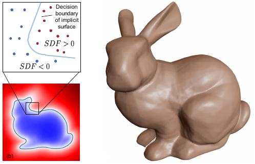
3D point $x$, we can precompute the minimum distance from $x$ to any
point on our model, call it $\phi(x).$ The term above is just
$\phi({^OX^Wp^{s_i}}).$ This function of 3D space, sometimes called a
distance
field, and the closely related signed distance function (SDF) and
level sets
are a common representation in geometric modeling. And they are
precisely what we need to quickly compute the cost from many scene
points.
Contour plot of
the distance function for our point-based representation of the rectange
(left), and the signed distance function for our "mesh-based" 2D
rectangle. The smoother distance contours in the mesh-based
representation can help alleviate some of the local minima problems we
observed above.A
visualization of a "signed distance function" (SDF) representation of 3D
geometry. Reproduced with permissions from
Park19.
As the figure I've included above suggests, we can use the
precomputed distance functions to represent the minimum distance to a
mesh model instead of just a point cloud. And with some care, we can
define alternative distance-like functions in 3D space that have smooth
subgradients which can work better with nonlinear optimization. There
is a rich literature on this topic; see Osher03 for a nice
reference.
Global optimization
Is there any hope of exploiting the beautiful structure that we found
in the pose estimation with known correspondences with an algorithm that
searches for correspondences and pose simultaneously?
There are some algorithms that claim global optimality for the ICP
objective, typically using a branch and bound strategy
Gelfand05+Mellado14+Yang15, but we have been disappointed
with the performance of these on real point clouds. We proposed another,
using branch and bound to explicitly enumerate the correspondences with a
truncated least-squares objective, and a tight relaxation of the SE(3)
constraintsIzatt17b, but this method is still limited to
relatively small problems.
In recent work, TEASER Yang20a takes a different
approach, using the observation that truncated least squares can be
optimized efficiently for the case of scale and translation. For
rotations, they solve a semidefinite (SDP) relaxation of the truncated
least-squares objective. This relaxation is not guaranteed to be tight,
but (like all of the convex relaxations we describe in this chapter), it
is easy to certify after the fact whether the optimal solution satisfied
the original constraints. And the SDP relaxation of the quadratic
rotation matrix constraints can
be surprisingly effectiveSaunderson15!
Non-penetration and "free-space" constraints
We've explored two main lineages of algorithms for the pose estimation
-- one based on the beautiful SVD solutions and the other based on
nonlinear optimization. As we will see, non-penetration and free-space
constraints are, in most cases, non-convex constraints, so are a better
match for the nonlinear optimization approach. But there are some examples
of convex non-penetration constraints (e.g., when points must not penetrate
a half-plane) and it is possible to include these in our convex
optimization approach. I'll illustrate both versions here with a simple
example.
Non-penetration via nonlinear
optimization
For simplicity, I will restrict this example to 2D, where we can
parameterize the rotation matrices: $$R(\theta) = \begin{bmatrix}
\cos(\theta) & -\sin(\theta) \\ \sin(\theta) & \cos(\theta)
\end{bmatrix},$$ and will solve the problem with known correspondences.
Please do remember, though, that we can also include the correspondence
search in the nonlinear optimization framework.
Let's solve the following optimization: \begin{align*} \min_{p,\theta}
\quad & \sum_i \| p + R(\theta) \: {}^Op^{m_{c_i}} - p^{s_i} \|^2, \\
\subjto \quad & {}^W p^{m_i} \ge 0, \quad \forall i \in [1, N_m].
\end{align*} In order to add the nonlinear costs and constraints, we use
pass a python function and the decision variables to be bound with that
function to the MathematicalProgramAddCost and
AddConstraint methods. I've provided an implementation in
this notebook:
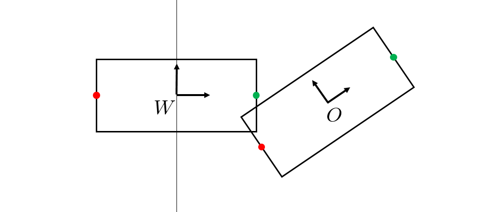
The solution to
the constrained pose estimation problem with known correspondences. I
have added constraints that both the $x$ and $y$ positions of all of the
points in the estimated pose must be greater than $0$ in the world frame
(as illustrated by the green lines). The red scene points are in
penetration, but the solver returns the pose illusutrated by the blue,
which satisfies the constraints.
Non-penetration via convex optimization
For a convex parameterization of the rotation matrices in this 2D
example, we can leverage our convenient form of the rotation matrices:
$$R = \begin{bmatrix} a & -b \\ b & a \end{bmatrix}.$$ Recall that the
rotation matrix constraints for this form reduce to $a^2+b^2=1$. These
are non-convex constraints, but we can relax them to $a^2 + b^2 \le 1.$
This is almost exactly the problem we visualized in this earlier example, except that we will
add translations here. The relaxation is exactly changing the non-convex
unit circle constraint into the convex unit disk constraint. Based on
that visualization, we have reason to be optimistic that the unit disk
relaxation could be tight.
Let's solve the following optimization: \begin{align*} \min_{p,a,b}
\quad & \sum_i \| p + R \: {}^Op^{m_{c_i}} - p^{s_i} \|^2, \\ \subjto
\quad & a^2 + b^2 \le 1, \\ & {}^W p^{m_i} \ge 0, \quad \forall i \in [1,
N_m], \end{align*} where $R$ depends on $a, b$ as above. Just as the
addition of constraints forced us to move from the pseudo-inverse solution
to a numerical optimization-based solution in the last chapter, the
solution to this problem is no longer given simply by SVD. As formulated,
this optimization falls under the category of a Second-Order Cone Program
(SOCP), though we need to use a slack variable to put it into the standard
form with a linear objective.
Please be careful. Now that we have a constraint that depends on $p$,
our original approach to solving for $R$ independently is no longer valid
(at least not without modification). I've provided a simple implementation in the notebook.
The convex
approximation to the constrained pose estimation problem with known
correspondences. I have added constraints that both the $x$ and $y$
positions of all of the points in the estimated pose must be greater than
$0$ in the world frame (as illustrated by the green
lines).
This is a slightly exaggerated case, where the scene points are really
pulling the box into the constraints. We can see that the relaxation is
not tight in this situation; the box is being shrunk slightly to
explain the data.
Constrained optimizations like this can be made relatively efficient,
and are suitable for use in an ICP loop for modest-sized point clouds. But
the major limitation is that we can only take this approach for convex
non-penetration constraints (or convex approximations of the constraints),
like the "half-plane" constraints we used here. It is probably not very
suitable for non-penetration between two objects in the scene.
For the record, the fact that I was able to easily add this example
here is actually pretty special. I don't know of another toolbox that
brings together the advanced optimization algorithms with the geometry /
physics / dynamical systems in the way that Drake does.
Free space constraints as non-penetration constraints
There is another beautiful idea that I first saw in
Schmidt15...
The rays
cast from the camera to the depth returns define a "free space obstacle"
that other objects should not penetrate.
Ultimately, as much as I prefer the convex formulations with their
potential for deeper understanding (by us) and for stronger guarantees (for
the algorithms), the ability to add non-penetration constraints and
free-space constraints is simply too valuable to ignore. Deep learning
methods can now often provide a good initial guess, which can mitigate some
of the concerns about local minima. I hope that, if you come back to these
notes in a year or two, I will be able to report that we have strong
results for these more complex formulations. But for now, in most
applications, I will steer you towards the nonlinear optimization
approaches and taking advantage of these constraints.
Tracking
Putting it all together
Now we can put all of the pieces together. In the notebook, I've
created an example with the mustard bottle in one bin. First, I use ICP to
localize its pose. Then, I plan a simple trajectory like we did in the
last chapter to pick it up and place it in the second bin. Finally, I use
differential inverse kinematics to execute it. Very satisfying!
Looking ahead
Although I very much appreciate the ability to think rigorously about
these geometric approaches, we need to think critically about whether we are
solving for the right objectives.
Even if we stay in the realm of pure geometry, it is not clear that a
least-squares objective with equal weights on the points is correct. Imagine
a tall skinny book laying flat on the table -- we might only get a very
small number of returns from the edges of the book, but those returns
contain proportionally much more information than the slew of returns we
might get from the book cover. It is no problem to include relative weights
in the estimation objectives we have formulated here, but we don't yet have
very successful geometry-based algorithms for deciding what those weights
should be in any general way. (There has been a lot of research in this
direction, but it's a hard problem.)
Please realize, though, that as beautiful as geometry is, we are so far
all but ignoring the most important information that we have: the color
values! While it is possible to put color and other features into an
ICP-style pipeline, it is very hard to write a simple distance metric in
color space (the raw color values for a single object might be very
different in different lighting conditions, and the color values of
different objects can look very similar). Advances in computer vision,
especially those based on deep learning over the last few years, have
brought new life to this problem. When I asked my students recently "If
you had to give up one of the channels, either depth or color, which would
you give up?" the answer was a resounding "I'd give up depth; don't take
away my color!" That's a big change from just a few years ago. As recently
as 2019, in the Benchmark for 6D Object Pose Estimation (a nearly annual
competition), geometric pose estimation was still outperforming
deep-learning based approachesHodan20. But by the 2020
version of the challenge, deep learning had caught up.
But deep learning and geometry can (should?) work nicely together. The
winners in the 2020 version of the object pose estimation challenge used
deep learning to make the initial guess at the pose, but still used
geometry perception (a variant of ICP) and the depth channel for refining
the estimateHodan20.For another example, identifying
correspondences between point clouds has been a major theme in this chapter
-- and we haven't completely solved it. This is one of the many places
where the color values and deep learning have a lot to offer
Florence18a. We'll turn our attention to them soon!
Exercises
How many points do you need?
Consider the problem of point cloud registration with known
correspondences. Points can be directly mapped to corresponding model points to
specify the position and orientation of an object in the scene. In most cases, we have far more points
than we have decision variables on the object's pose. Therefore, treating each point
correspondence as an equality constraint would make the problem over-constrained.
This raises a natural question:
What is the minimum number of points that can uniquely
specify the pose of an object in 2D? Provide a brief justification.
What is the minimum number of points that can uniquely
specify the pose of an object in 3D? Provide a brief justification.
(HINT: How might your answers change if point correspondences were unknown?)
Rotational symmetries
We have a beautiful formulation for the point cloud registration
problem with known correspondences -- it has a quadratic objective and
(with the determinant constraint relaxed) a quadratic equality constraint.
Sometimes we have objects that are rotationally symmetric -- think of box
that is a perfect cube. How can the quadratic objective capture a problem
where there should be equally good solutions at rotations that are 90
degrees apart?
ICP with random initializations
If you run the ICP example code which has randomized object geometry
and ground truth object pose, you can't help but notice that the algorithm
does a quite reasonable job of estimating translation, but (at least for
the geometries I've generated here) does a fairly lousy job with rotation.
One mitigation is to run ICP multiple times with different initial
estimates of the rotation. This is a reasonable strategy for any
nonconvex optimization problem with local minima, but is particularly
useful here since even when the point clouds are quite complex, the
dimensionality of the search space is low. In particular, we can generate
a reasonable coverage of 2D or even 3D rotations with a modest number of
samples (for 3D, consider using
UniformlyRandomRotationMatrix). Furthermore, running ICP
from multiple initial conditions can be done in parallel.
Try implementing ICP from multiple initial estimates $\hat{X}^O$,
sampling only in rotation. If you only keep the best one (lowest
estimation error), then how much does it improve the performance over a
single ICP run?
Point Registration with Fixed Rotation
Consider the case of point registration where the rotation component
of $X^O$ is known, but not the translation. (In other words, the opposite
of Example 4.2.)
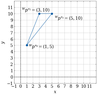
Specifically, say your scene points ${}^WX^C{}^Cp^{s_i}={}^Wp^{s_i}$
are defined as follows:
$$ \begin{aligned} {}^Wp^{s_0}&=(1,5) \\ {}^Wp^{s_1}&=(3,10) \\
{}^Wp^{s_2}&=(5,10) \end{aligned} $$ Which can be plotted as follows:
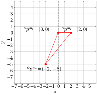
And your model points are defined as follows:
$$ \begin{aligned} {}^Op^{m_0}&=(-2,-5) \\ {}^Op^{m_1}&=(0,0) \\
{}^Op^{m_2}&=(2,0) \end{aligned} $$ Which can be plotted as follows:
As you can see, both triangles are in the same orientation, so $R^O=
\begin{bmatrix} 1 & 0 \\ 0 & 1 \end{bmatrix}$. However, we still need
to solve for the translation component of $X^O$.
(In this example, we can easily separate translation and rotation
because the orientation of the model already matches the scene, but
this decoupling actually works in the general case as well. See the
explanation following Example 4.2 in the textbook.)
What are the decision variables in this optimization problem? Be
specific.
What is the value of the objective function for $p^O = (0,0)$? What
about (3,10)? And (6,12)?
If you plotted the objective function as a function
of your decision variables, what shape would it be? Explain the
significance of this.
Consider the general case where rotation is fixed with an equal number of scene and model points.
We only need to find the translational component. Solving this optimization problem,
what quantity do we find for each decision variable? Your solution should be correct even when the model and scene points cannot be perfectly aligned (e.g. noise).
(HINT: We want to minimize the squared distance of all the transformed scene points compared to their corresponding model points.)
Planar Two-Point ICP
We saw that ICP has many local minima. But what are these local
minimas, and can we say something about how wrong our initial guess has
to be until we arrive at one of these local minima? Although the analysis
can get complicated for general geometry, let's start by analyzing a
simple example of a planar two-point ICP.
The model points and the scene points in their corresponding frame are given as:
The true correspondence is given by their numbering, but note that we
don't know the true correspondence - ICP simply determines it based on
nearest neighbors. Given our vanilla-ICP cost (sum of pairwise distances
squared), we can parametrize the 2D pose $X^O$ with $p_x,p_y,a,b$ and
write down the resulting optimization as:
When the initial guess for the pose results in the correct
correspondences based on nearest-neighbors, show that the ICP cost is
minimum when $p_x,p_y,b=0$ and $a=1$. Describe the set of initial
poses that results in convergence to the true solution.
When the initial guess results in a flipped correspondence, show
that ICP cost is minimum when $p_x,p_y,b=0$ and $a=-1$. Describe the
set of initial poses that results in convergence to this incorrect
solution.
Remember that correspondence need not be one-to-one. In fact they
are often not when computed based on nearest-neighbors. By constructing
the data matrix $W$, show that when both scene points correspond to one
model point, ICP gets stuck and does not achieve zero-cost. What happens on the next iteration of ICP?
(HINT: You may assume that doing SVD on a zero matrix leads to identity matrices
for $U$ and $V$).
Bunny ICP
For this exercise, you will implement the ICP algorithm to match
pointclouds of two Stanford bunnies. You will work exclusively in . You will be asked to complete the
following steps:
Implement a method to compute the least-squares transform given
the correspondences.
Implement the ICP algorithm using the least square transform
method from part a.
RANSAC
For this exercise, you will remove the environmental background from
the Stanford bunny pointcloud using the RANSAC algorithm. You will work
exclusively in . You will be asked to complete the
following steps:
Implement the RANSAC algorithm.
Use the RANSAC algorithm to remove the planar surface from the
scene point cloud.
Outliers in ICP
In this question you'll explore a technique for handling outliers in
ICP and think through how the distance metric impacts the robustness of
ICP to outliers. There are two parts to this question and each part has
three subquestions.
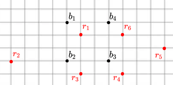
Consider the setting visualized below. Here the model points are
given in black and labeled as $b_{i}$ and the scene points are given
in red and labeled as $r_{j}$.
Let's consider a possible algorithm for handling the outliers in the
scene.
First, write down each of the correspondence, i.e the ($b_{i},
r_{j}$) pairs. Next, compute the ICP error, the sum of the pairwise squared
distances between each of these correspondences.
Suppose that you are told that $\frac{1}{3}$ of the scene
points are outliers. Using the pairwise distances between each
$b_{i}$ and $r_{j}$, which two scene points $r_{j}$ could you
detect as the most likely outliers?
Discarding the two proposed outlier scene points, compute the
new ICP error.
This is the basic intuition behind the Trimmed ICP
algorithm!
The optimization in ICP captures the distance between two sets of
points as the sum of pairwise Euclidean squared distances. As a thought
experiment: another possible distance metric (which isn't as
optimization friendly) is the one-way Hausdorff distance. Stated
simply, given that an adversary picks a point on one shape, the one-way Hausdorff distance is the distance you
are forced to travel to get to the closest point on the other shape.
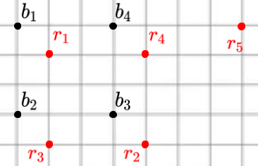
We could consider two schemes: Scheme 1) The adversary picks the scene point and thus you
pick the model point that is closest to this scene point. Scheme 2) The adversary picks the model point and thus you
pick the scene point that is closest to this model point.
Which is more robust to outliers? Let's explore through a 2D example.
Again, the model points are given in black and labeled as $b_{i}$ and
the scene points are given in red and labeled as $r_{j}$.
Lets consider scheme 1. I, as the adversary, pick the scene
point $r_{5}$. Whats the nearest model point $b_{i}$ you can pick?
Whats the distance to this model point?
Now in scheme 2, I pick the model point $b_{1}$. What's the
nearest scene point $r_{j}$ that you can pick? What's the distance
to this scene point?
From this, which scheme was more robust to the outlier?
Pose Estimation
Let's go back to the example from Chapter 3, but relax the assumption
that we have the pose of the red foam brick. You will be given a
simulated raw pointcloud from our previous setup from a depth camera.
Your task is to perform segmentation on this raw pointcloud data, and
perform ICP to estimate the pose of the brick. You will work exclusively
in
. You will be asked to complete the
following steps:
Perform segmentation on the raw pointcloud to remove the
background.
Use our class ICP implementation to correctly estimate the pose of
the red foam brick.
Composing Signed Distance Functions (SDFs)
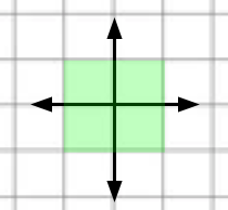
In this problem we will explore signed distance functions and their composition! As a reminder, the signed distance function of a set gives the minimum distance of a point $p$ to the boundary of that set, where the sign of the value is based on whether the point $p$ is inside or outside the boundary. Points that are on the interior of the boundary are negative. and points that are on the exterior of the boundary are positive.
For a 2D example, consider the green box visualized below. The center of the box, at the origin, has a signed distance value of -1, since it is distance one from any of the edges of the box and it lies on the interior of the box. Points along the perimeter of the box have a signed distance value of 0. Any points outside the box have a signed distance value of $+d$ where $d$ is the smallest distance between that point and the perimeter of the box.
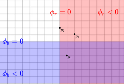
In the figure below we draw two objects: a shaded red object and a shaded blue object (the purple region is two objects overlapping and the objects should be treated as infinite half planes). Let $\phi_r(p)$ be the signed distance value of a point $p$ to boundary of the red object and $\phi_b(p)$ be the signed distance value of point $p$ to the boundary blue object. As an example $\phi_b(p_0) = -3, \phi_b(p_1) = +2$.
First, lets consider a new region defined as the union of red object and the blue object. Let $\phi_{r \cup b}(p)$ be the signed distance value of a point $p$ to this new boundary. Compute: $\phi_{r \cup b}(p_{0}), \phi_{r \cup b}(p_{1}), \phi_{r \cup b}(p_{2})$.
Next, lets consider a new region defined as the intersection of the red object and the blue object (hence the purple object). Let $\phi_{r \cap b}(p)$ be the signed distance value of a point $p$ to this new boundary. Compute: $\phi_{r \cap b}(p_{0}), \phi_{r \cap b}(p_{1}), \phi_{r \cap b}(p_{2})$.
Using your experience from part (a), write an expression for computing the signed distance value for any point $p$ in our 2D space to the union of the red and blue objects. Your expression should be in terms of $\phi_r(p)$ and $\phi_b(p)$. We encourage you to think in terms of cases based on what region the point is in. HINT: Write a case statement that cases on the 4 regions, then try to reduce it to 2 cases with a clean math expression.
Using your experience from part (b), write an analogous expression for computing the signed distance value for any point $p$ to the intersection of the red and blue objects (i.e. the purple region). Your expression should be in terms of $\phi_r(p)$ and $\phi_b(p)$, and it can be written considering only 2 cases.
One incorrect method to compute the SDF value for the union of two objects is to simply take the minimum of the SDF value for each of the objects. (It is worth taking a minute to convince yourself why this method is incorrect!). While this method can produce the incorrect distance, it will produce a value with the correct sign (again, convince yourself this is true!).
Therefore, this "incorrect" method can tell us if we are in penetration or out of penetration for the union of our set of objects. This makes it useful for computing a non-penetration constraint! We'll refer to the SDF generated by this "incorrect-but-useful" method as Penetration-Constraint-SDF.
Let's see how we can use this!
As discussed in class, for rigid objects, we can precompute the SDF
for the object, which enables us to greatly speed up computations.
However, if we are dealing with an articulated body, such as a robot arm,
where the configuration of the arm is dependent on the joint values, we
can no longer precompute the SDF. Recomputing this "global" SDF every
time the robot's configuration changes gets very expensive. (By global we
mean an SDF of the entire articulated body.)
Instead, the DART (Dense Articulated Real-Time Tracking)
Schmidt15 algorithm considers that for each link in the
articulated body, we have a "local" SDF. A local SDF gives the signed
distance value to a point in the link's coordinate frame. Because we are
operating in the link's coordinate frame, we can precompute these local
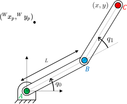
SDFs. Consider that we have our favorite, planar two-link arm, picture
below. Given $q_{0}, q_{1}$ and the precomputed local SDFS for each of
the links (link AB, link BC), briefly describe how you could compute the
value of the global Penetration-Constraint-SDF for a point $(^{W}x_{p},
^{W}y_{p})$.
,
Manipulating Assets In The Wild With Geometric Sensing
In this exercise, we will build upon Exercise 3.14 from the previous chapter. This time,
you will program the robot to pick and place letter assets from your initials without assuming that you know the initial pose of the assets by using depth
cameras and geometric sensing. You will work exclusively in .
You will be asked to complete the following steps:
Create a scenario with the robot, table, your initials, and three RGB-D sensors.
Use the RGB-D sensors to get pointclouds of the initials.
Use ICP to estimate the pose of the initials in the world.
Use the estimated poses to pick and place the initials with your Differential IK controller from Exercise 3.14
References
Krishna Shankar and Mark Tjersland and Jeremy Ma and Kevin Stone and Max Bajracharya,
"A learned stereo depth system for robotic manipulation in homes",
IEEE Robotics and Automation Letters, vol. 7, no. 2, pp. 2305--2312, 2022.
Chris Sweeney and Greg Izatt and Russ Tedrake,
"A Supervised Approach to Predicting Noise in Depth Images",
Proceedings of the IEEE International Conference on Robotics and Automation , May, 2019.
[ link ]
Jeong Joon Park and Peter Florence and Julian Straub and Richard Newcombe and Steven Lovegrove,
"DeepSDF: Learning Continuous Signed Distance Functions for Shape Representation",
Proceedings of the IEEE International Conference on Computer Vision and Pattern Recognition (CVPR) , June (To Appear), 2019.
[ link ]
Ben Mildenhall and Pratul P Srinivasan and Matthew Tancik and Jonathan T Barron and Ravi Ramamoorthi and Ren Ng,
"Nerf: Representing scenes as neural radiance fields for view synthesis",
Communications of the ACM, vol. 65, no. 1, pp. 99--106, 2021.
Berthold K.P. Horn,
"Closed-form solution of absolute orientation using unit quaternions",
Journal of the Optical Society of America A, vol. 4, no. 4, pp. 629-642, April, 1987.
Andriy Myronenko and Xubo Song,
"On the closed-form solution of the rotation matrix arising in computer vision problems",
arXiv preprint arXiv:0904.1613, 2009.
Robert M Haralick and Hyonam Joo and Chung-Nan Lee and Xinhua Zhuang and Vinay G Vaidya and Man Bae Kim,
"Pose estimation from corresponding point data",
IEEE Transactions on Systems, Man, and Cybernetics, vol. 19, no. 6, pp. 1426--1446, 1989.
Marius Muja and David G Lowe,
"Flann, fast library for approximate nearest neighbors",
International Conference on Computer Vision Theory and Applications (VISAPP’09) , vol. 3, 2009.
Bertram Drost and Markus Ulrich and Nassir Navab and Slobodan Ilic,
"Model globally, match locally: Efficient and robust 3D object recognition",
2010 IEEE computer society conference on computer vision and pattern recognition , pp. 998--1005, 2010.
Tomás Hodan and Martin Sundermeyer and Bertram Drost and Yann Labbé and Eric Brachmann and Frank Michel and Carsten Rother and Jirí Matas,
"BOP Challenge 2020 on 6D Object Localization",
European Conference on Computer Vision Workshops (ECCVW), 2020.
M.A. Fischler and R.C. Bolles,
"Random Sample Consensus: A Paradigm for Model Fitting with Applications to Image Analysis andd Automated Cartography",
Communications of the Association for Computing Machinery (ACM) , vol. 24, no. 6, pp. 381--395, 1981.
Heng Yang and Jingnan Shi and Luca Carlone,
"Teaser: Fast and certifiable point cloud registration",
arXiv preprint arXiv:2001.07715, 2020.
Pat Marion and Peter R. Florence and Lucas Manuelli and Russ Tedrake,
"A Pipeline for Generating Ground Truth Labels for Real RGBD Data of Cluttered Scenes",
International Conference on Robotics and Automation (ICRA), Brisbane, Australia, May, 2018.
[ link ]
Anh Nguyen and Bac Le,
"3D point cloud segmentation: A survey",
2013 6th IEEE conference on robotics, automation and mechatronics (RAM) , pp. 225--230, 2013.
Andriy Myronenko and Xubo Song,
"Point set registration: Coherent point drift",
IEEE transactions on pattern analysis and machine intelligence, vol. 32, no. 12, pp. 2262--2275, 2010.
Wei Gao and Russ Tedrake,
"FilterReg: Robust and Efficient Probabilistic Point-Set Registration using Gaussian Filter and Twist Parameterization",
Conference on Computer Vision and Pattern Recognition (CVPR), June, 2019.
[ link ]
Andrew W Fitzgibbon,
"Robust registration of 2D and 3D point sets",
Image and vision computing, vol. 21, no. 13-14, pp. 1145--1153, 2003.
Stanley Osher and Ronald Fedkiw,
"Level Set Methods and Dynamic Implicit Surfaces", Springer
, 2003.
Natasha Gelfand and Niloy J Mitra and Leonidas J Guibas and Helmut Pottmann,
"Robust global registration",
Symposium on geometry processing , vol. 2, no. 3, pp. 5, 2005.
Nicolas Mellado and Dror Aiger and Niloy J Mitra,
"Super 4pcs fast global pointcloud registration via smart indexing",
Computer Graphics Forum , vol. 33, no. 5, pp. 205--215, 2014.
Jiaolong Yang and Hongdong Li and Dylan Campbell and Yunde Jia,
"Go-ICP: A globally optimal solution to 3D ICP point-set registration",
IEEE transactions on pattern analysis and machine intelligence, vol. 38, no. 11, pp. 2241--2254, 2015.
Gregory Izatt and Hongkai Dai and Russ Tedrake,
"Globally Optimal Object Pose Estimation in Point Clouds with Mixed-Integer Programming",
International Symposium on Robotics Research, Dec, 2017.
[ link ]
James Saunderson and Pablo A Parrilo and Alan S Willsky,
"Semidefinite descriptions of the convex hull of rotation matrices",
SIAM Journal on Optimization, vol. 25, no. 3, pp. 1314--1343, 2015.
Tanner Schmidt and Richard Newcombe and Dieter Fox,
"DART: dense articulated real-time tracking with consumer depth cameras",
Autonomous Robots, vol. 39, no. 3, pp. 239--258, 2015.
Peter R. Florence* and Lucas Manuelli* and Russ Tedrake,
"Dense Object Nets: Learning Dense Visual Object Descriptors By and For Robotic Manipulation",
Conference on Robot Learning (CoRL) , October, 2018.
[ link ]

 Please make sure you spend a minute
with the MeshCat visualization (available
here). You'll see a camera and the camera frame, and you'll see the
mustard bottle as always... but it might look a little funny. That's
because I'm displaying both the ground truth mustard bottle model
and the point cloud rendered from the cameras. You can use the
MeshCat GUI to uncheck the ground truth visualization (image right), and you'll be able to see just the point cloud.
Please make sure you spend a minute
with the MeshCat visualization (available
here). You'll see a camera and the camera frame, and you'll see the
mustard bottle as always... but it might look a little funny. That's
because I'm displaying both the ground truth mustard bottle model
and the point cloud rendered from the cameras. You can use the
MeshCat GUI to uncheck the ground truth visualization (image right), and you'll be able to see just the point cloud.
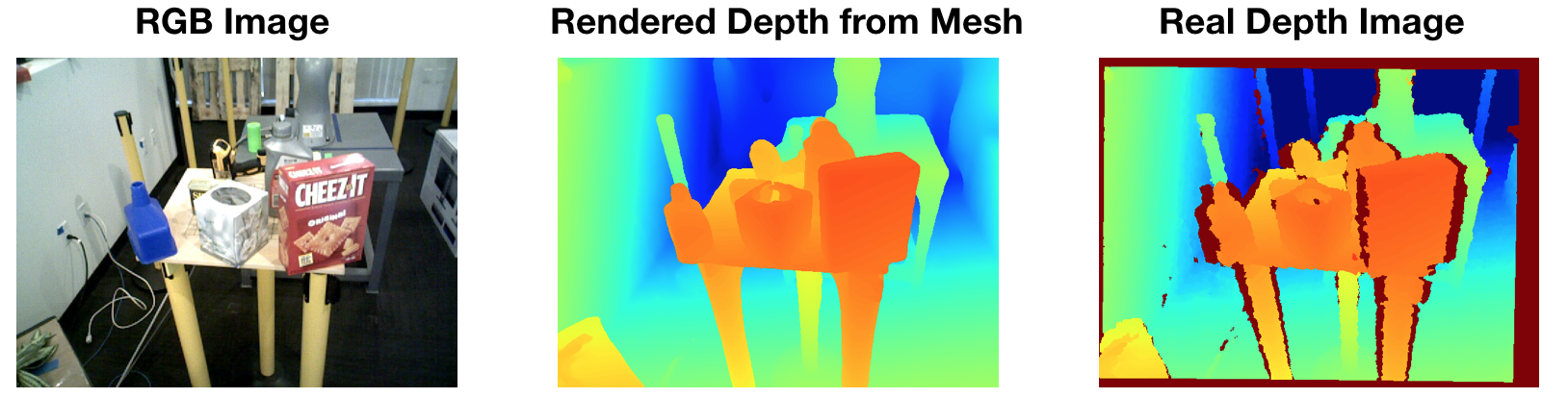

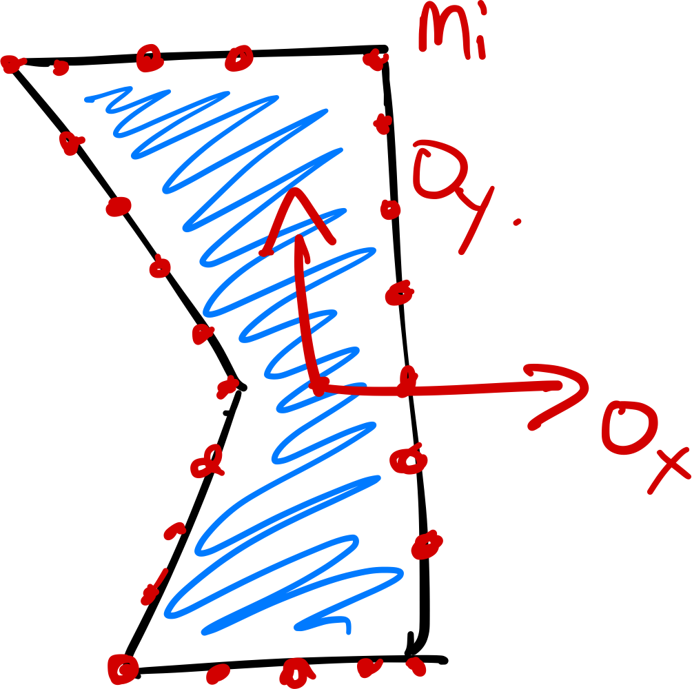 One very natural and well-studied
formulation of this problem comes from the literature on point cloud
registration (also known as point set registration or scan matching).
Given two point clouds, point cloud registration aims to find a rigid
transform that optimally aligns the two point clouds. For our purposes,
that suggests that our "model" for the object should also take the form of a
point cloud (at least for now). We'll describe that object with a list of
model points, $m_i$, with their pose described in the object frame:
$^OX^{m_i}.$
One very natural and well-studied
formulation of this problem comes from the literature on point cloud
registration (also known as point set registration or scan matching).
Given two point clouds, point cloud registration aims to find a rigid
transform that optimally aligns the two point clouds. For our purposes,
that suggests that our "model" for the object should also take the form of a
point cloud (at least for now). We'll describe that object with a list of
model points, $m_i$, with their pose described in the object frame:
$^OX^{m_i}.$ 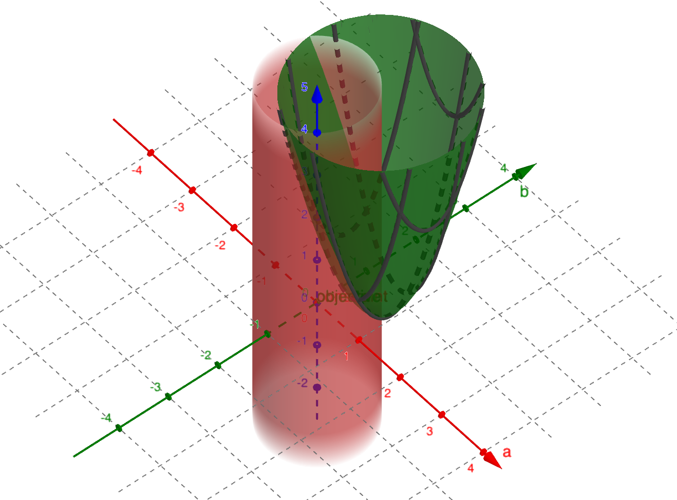


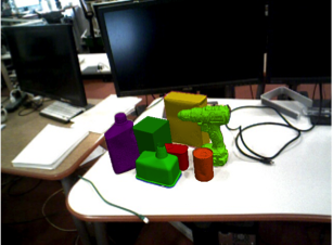
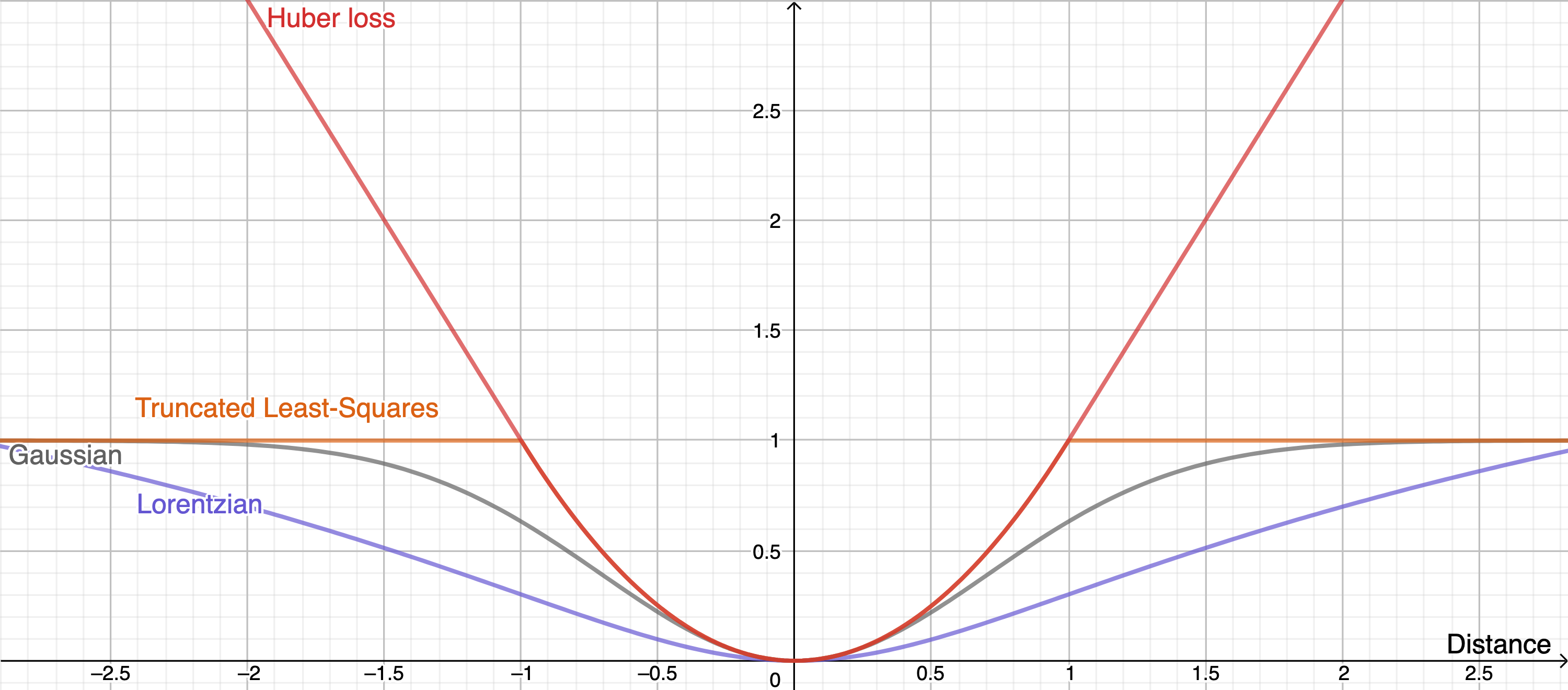
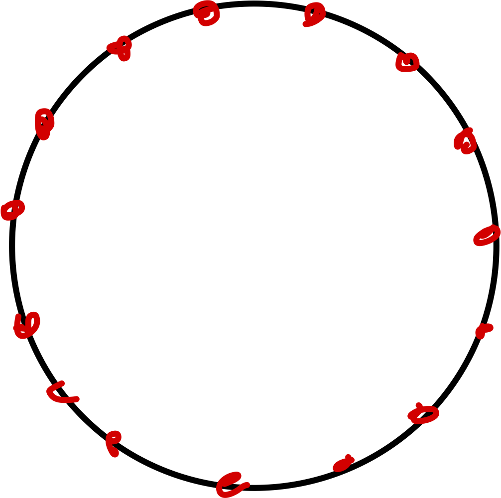 As a thought experiment, consider
the problem where all of our model points lie on a perfect circle. For
any one scene point $i$, in the rotation-only optimization, the worst
case is when our estimate $\theta$ is 180 degrees ($\pi$ radians) away
from the optimal solution. The cost for that point would be $4r^2$,
where $r$ is the radius of the circle. In fact, using the law of
cosines, we can actually write the squared distance for the point for
any error, $\theta_{err} = \theta - \theta^*,$ as $$\text{distance}^2 =
r^2 + r^2 - 2 r^2 \cos\theta_{err}.$$ And in the case of the circle,
every other model point contributes the same cost. This is not a convex
function, but every minima is a globally optimal solution (just wrapped
around by $2\pi$).
As a thought experiment, consider
the problem where all of our model points lie on a perfect circle. For
any one scene point $i$, in the rotation-only optimization, the worst
case is when our estimate $\theta$ is 180 degrees ($\pi$ radians) away
from the optimal solution. The cost for that point would be $4r^2$,
where $r$ is the radius of the circle. In fact, using the law of
cosines, we can actually write the squared distance for the point for
any error, $\theta_{err} = \theta - \theta^*,$ as $$\text{distance}^2 =
r^2 + r^2 - 2 r^2 \cos\theta_{err}.$$ And in the case of the circle,
every other model point contributes the same cost. This is not a convex
function, but every minima is a globally optimal solution (just wrapped
around by $2\pi$).