Pset #2 part 1 of 3: Iterative Closest Point (ICP)
In this problem you will implement the iterative closest point (ICP) algorithm. As discussed in class, ICP aims to find an optimal transform between two point clouds. It does this by iteratively solving \begin{gather} \min_{R, t, c} \ \ \ \sum_{i} \| R s_i + t - m_{c_i}\|_2^2 \\ s.t. \ \ \ R^T = R^{-1}, \mathrm{det}(R) = 1 \\ \end{gather} where $s_i$ are the points in the scene point cloud, $m_i$ are the points in the model point cloud, and $c_i$ is the integer index of the point in the $m$ that corresponds most closely with the $i$th point in the scene.
This is a very hard and non-convex problem, so instead of solving the optimization in one step, the algorithm alternates between solving for $\{R, t\}$ and $c$ separately.
In this problem you will implement each individual optimization, as well as the whole iterative algorithm. You will also explore how different parameters affect the overall performance.
For more references on ICP, check out the original paper by Besl and McKay, and this slide deck by Pieter Abbeel.
# Run this first! Imports stuff to be used in this notebook.
%reload_ext autoreload
%autoreload 2
import meshcat
import meshcat.geometry as g
import numpy as np
from iterative_closest_point import (nearest_neighbors,
                                     least_squares_transform,
                                     icp,
                                     repeat_icp_until_good_fit,
                                     visualize_icp,
                                     clear_vis)
1. Finding the Nearest Neighbors
The first step of ICP is optimizing $c$ assuming $R$ and $t$ are known.
\begin{align*} c_i = \underset{j}{\arg\min} \ \ \| R s_i + t - m_j\|_2^2 \\ \end{align*}This is also known as a nearest neighbors search.
Finish filling out the function nearest_neighbors in iterative_closest_point.py. You might want to look into this sklearn library. Assume the inputs to this function have already been transformed by $R$ and $t$.
%reload_ext autoreload
%autoreload 2
from sklearn.neighbors import NearestNeighbors

scene_point_cloud = np.array([[0, 0, 0],
                              [1, 2, 3],
                              [10, 9, 8],
                              [-3, -4, -5]])

model_point_cloud = np.array([[10, 9, 8],
                              [-3, -4, -5],
                              [1, 2, 3],
                              [0, 0, 0]])


distances, indices = nearest_neighbors(scene_point_cloud, model_point_cloud)

print("distances:", distances)
print("indices:", indices)
2. Finding the Least Squares Transform
The next step is solving for $R$ and $t$ given $c$. In class we discussed a way to do that using SVD. Define the "center of mass" of the model points and scene points as
\begin{align*} \mu_m = \frac{1}{N_s} \sum_i m_{c_i}, \\ \mu_s = \frac{1}{N_s} \sum_i s_i \end{align*}where $N_s$ is the number of points in the scene point cloud.
To solve for the optimal $R = R^*$, make use of SVD.
\begin{gather} W = \sum_i (m_{c_i} - \mu_m) (s_i - \mu_s)^T \\ U \Sigma V^T = \text{SVD}(W) \\ R^* = U V^T \end{gather}Then $t^*$ is simply
\begin{align*} t^* = \mu_m - R^* \mu_s \end{align*}Finishing filling in the function least_squares_transform in iterative_closest_point.py to calculate $R^*$ and $t^*$ given $c$. Assume that the inputs have already taken $c$ into account (i.e. just compare the input point clouds directly). Instead of returning $R^*$ and $t^*$ separately, return a single homogenous transformation matrix.
Important note: Sometimes this formulation of $R^*$ gives a Householder reflection matrix instead of a rotation matrix. If this is the case, which can be checked if the determinant of $R^*$ is -1, you must negate the third column of $V$, then recompute $R^*$.
%reload_ext autoreload
%autoreload 2

scene_point_cloud = np.array([[1, 1, 1],
                              [2, 2, 2],
                              [3, 3, 3],
                              [4, 4, 4]])

model_point_cloud = np.array([[2, 2, 2],
                              [3, 3, 3],
                              [4, 4, 4],
                              [5, 5, 5]])

X_MS = least_squares_transform(scene_point_cloud, model_point_cloud)

print("Transformation:")
print(X_MS.matrix())
3. The ICP Algorithm
Now that you have solved the two separate optimizations, it's time to put them together in ICP. The basic steps are:
- Given an initial $R$ and $t$, calculate $c$ (the nearest neighbors)
- Use $c$ to solve for a better $R$ and $t$
- If the new mean error, defined as the mean of the distances of the nearest neighbors, hasn't changed since the last iteration by some amount, terminate the iterations. Otherwise go back to step 1 and repeat.
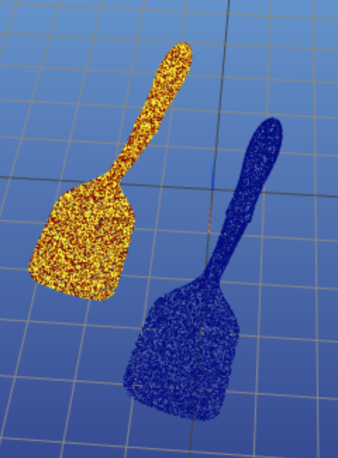
Finish filling out the icp function in iterative_closest_point.py. Run the cells below to test your code. The red point cloud is the model and the blue is the scene your robot observes. ICP will produce a transform that when applied to the scene point cloud, should align it with the model point cloud. The attempted alignment is the yellow point cloud. See the image below for the desired behavior with a spatula.
# First start meshcat for visualization - this only has to be run once

# If you interrupt the kernel of this notebook, you'll need to run this cell again to
# restart the meshcat server, and then refresh the visualization window.

# This will open a mesh-cat server in the background, click on the url to display
# visualization in a separate window.
vis = meshcat.Visualizer()

# Duplicate the visualization inside this cell (at a lower resolution).
# vis.jupyter_cell()
# Load in all of the point clouds needed for the rest of this notebook. These only have
# to be loaded once.

# All of these point clouds have shape (10000, 3) -> 10000 points in 3D space

# Spatula
spatula_model = np.load("resources/spatula_model.npy")
spatula_translation = np.load("resources/spatula_simple_translation.npy")
spatula_rotation = np.load("resources/spatula_simple_rotation.npy")
spatula_scene = np.load("resources/spatula_scene.npy")

# Sugar Box
sugar_box_model = np.load("resources/sugar_box_model.npy")
sugar_box_translation = np.load("resources/sugar_box_simple_translation.npy")
sugar_box_rotation = np.load("resources/sugar_box_simple_rotation.npy")
sugar_box_scene = np.load("resources/sugar_box_scene.npy")

# Apple
apple_model = np.load("resources/apple_model.npy")
apple_scene = np.load("resources/apple_scene.npy")
3.1 Spatula Matching
First test your implementation on a spatula. Because ICP shifts each point cloud to its centroid before trying to find a transform, small translations should work very well. Run the cell below (but make sure you've run meschat first!) to align a translated spatula to the model. The translation is 1 m in the x direction and 1 m in the y direction, so the final transform that ICP returns should be close to
\begin{align} \begin{bmatrix} 1 & 0 & 0 & 1 \\ 0 & 1 & 0 & 1 \\ 0 & 0 & 1 & 0 \\ 0 & 0 & 0 & 1 \end{bmatrix} \end{align}Use the default parameters of max_iterations = 20 and tolerance = 1e-3. Even though we know the transform, don't give it an initial guess. Note that the alignment probably won't be perfect, but it should be close.
%reload_ext autoreload
%autoreload 2

# Clear any point clouds already in meshcat.
clear_vis(vis)

# ICP expects Nx3 matrices, so we transpose the loaded point clouds.
X_MS, mean_error, num_iters = icp(spatula_translation, spatula_model)

print("Final transform:")
print(X_MS.matrix())
print("mean error:", mean_error)
print("total iterations:", num_iters)

# Visualize the point clouds in meshcat. Make sure you ran the cell initializing
# meshcat above.
# The model, scene and transformed scene point clouds are shown in red, blue and yellow,
# respectively.
# If ICP is implemented correctly, you should see the yellow point cloud aligned with the
# red point cloud.
visualize_icp(vis, spatula_translation, spatula_model, X_MS)
Once you think your algorithm works for this simple translation case, try running it on a 90 degree rotation of the spatula about the x-axis. There was no translation in this case, so what should the resulting transform be? Note that the alignment probably won't be perfect, but it should be close.
The code you ran above is in the function single_icp_run. Rather than copying the same code over and over again, just run that function now that you've seen how running it works. Once again, keep the default max_iterations and tolerance.
%reload_ext autoreload
%autoreload 2

clear_vis(vis)

X_MS, mean_error, num_iters = icp(spatula_rotation, spatula_model)

print("Final transform:")
print(X_MS.matrix())
print("mean error:", mean_error)
print("total iterations:", num_iters)

visualize_icp(vis, spatula_rotation, spatula_model, X_MS)
3.2 Box Matching
Now that you've seen ICP work for a spatula, which has a complicated geometry, try something simpler. Repeat the same experiments for a translated and rotated box. The transformations are the same as for the spatula. Please continue to use the default iteration limit and convergence tolerance.
%reload_ext autoreload
%autoreload 2

clear_vis(vis)

X_MS, mean_error, num_iters = icp(sugar_box_translation, sugar_box_model)

print("Final transform:")
print(X_MS.matrix())
print("mean error:", mean_error)
print("total iterations:", num_iters)

visualize_icp(vis, sugar_box_translation, sugar_box_model, X_MS)
%reload_ext autoreload
%autoreload 2

clear_vis(vis)

X_MS, mean_error, num_iters = icp(sugar_box_rotation, sugar_box_model)

print("Final transform:")
print(X_MS.matrix())
print("mean error:", mean_error)
print("total iterations:", num_iters)

visualize_icp(vis, sugar_box_rotation, sugar_box_model, X_MS)
Were the results what you expected? Take a look at the mean error from these two cases and compare it with the mean errors of the spatula in the same two cases. Remember that you're running the same code on both objects! If the results are different from the spatula runs, don't try to change your algorithm just yet. First we'll explore how changing some of the parameters affects performance.
3.3 Decreasing the Convergence Tolerance
The default convergence tolerance is 0.001, which means if the mean error of two consecutive iterations is less than 0.001, the algorithm stops. In the case with the rotated box, there is at least some overlap of the transformed observations and ground truth. What happens when you decrease the tolerance? Try different values ranging from 1e-3 to 1e-6. Do you notice a difference in both the spatula and box? For now, keep the maximum number of iterations 20 and don't give any initial guesses.
%reload_ext autoreload
%autoreload 2

clear_vis(vis)

# Change the tolerance parameter.
X_MS, mean_error, num_iters = icp(spatula_translation, spatula_model, tolerance=1e-3)

print("Final transform:")
print(X_MS.matrix())
print("mean error:", mean_error)
print("total iterations:", num_iters)

visualize_icp(vis, spatula_translation, spatula_model, X_MS)
%reload_ext autoreload
%autoreload 2

clear_vis(vis)

# Change the tolerance parameter.
X_MS, mean_error, num_iters = icp(spatula_rotation, spatula_model, tolerance=1e-3)

print("Final transform:")
print(X_MS.matrix())
print("mean error:", mean_error)
print("total iterations:", num_iters)

visualize_icp(vis, spatula_rotation, spatula_model, X_MS)
%reload_ext autoreload
%autoreload 2

clear_vis(vis)

# Change the tolerance parameter.
X_MS, mean_error, num_iters = icp(sugar_box_translation, sugar_box_model, tolerance=1e-3)

print("Final transform:")
print(X_MS.matrix())
print("mean error:", mean_error)
print("total iterations:", num_iters)

visualize_icp(vis, sugar_box_translation, sugar_box_model, X_MS)
%reload_ext autoreload
%autoreload 2

clear_vis(vis)

# Change the tolerance parameter.
X_MS, mean_error, num_iters = icp(sugar_box_rotation, sugar_box_model, tolerance=1e-3)

print("Final transform:")
print(X_MS.matrix())
print("mean error:", mean_error)
print("total iterations:", num_iters)

visualize_icp(vis, sugar_box_rotation, sugar_box_model, X_MS)
3.4 Increasing the Maximum Number of Iterations
Take a look at the number of iterations that are run in each of the cases above? How often are you hitting the limit? Now try increasing max_iterations. Independently change max_iterations and tolerance, still without any initial guesses. We suggest the following ranges for your parameters, but these aren't hard limits and you can experiment as you please.
20 $\leq$ max_iterations $\leq$ 500
1e-3 $\leq$ tolerance $\leq$ 1e-8
%reload_ext autoreload
%autoreload 2

clear_vis(vis)

# Change the max_iterations and tolerance parameters.
X_MS, mean_error, num_iters = \
    icp(spatula_translation, spatula_model, max_iterations=20, tolerance=1e-3)

print("Final transform:")
print(X_MS.matrix())
print("mean error:", mean_error)
print("total iterations:", num_iters)

visualize_icp(vis, spatula_translation, spatula_model, X_MS)
%reload_ext autoreload
%autoreload 2

clear_vis(vis)

# Change the max_iterations and tolerance parameters.
X_MS, mean_error, num_iters = \
    icp(spatula_rotation, spatula_model, max_iterations=20, tolerance=1e-3)

print("Final transform:")
print(X_MS.matrix())
print("mean error:", mean_error)
print("total iterations:", num_iters)

visualize_icp(vis, spatula_rotation, spatula_model, X_MS)
%reload_ext autoreload
%autoreload 2

clear_vis(vis)

# Change the max_iterations and tolerance parameters.
X_MS, mean_error, num_iters = \
    icp(sugar_box_translation, sugar_box_model, max_iterations=20, tolerance=1e-3)

print("Final transform:")
print(X_MS.matrix())
print("mean error:", mean_error)
print("total iterations:", num_iters)

visualize_icp(vis, sugar_box_translation, sugar_box_model, X_MS)
%reload_ext autoreload
%autoreload 2

clear_vis(vis)

# Change the max_iterations and tolerance parameters.
X_MS, mean_error, num_iters = \
    icp(sugar_box_rotation, sugar_box_model, max_iterations=20, tolerance=1e-3)

print("Final transform:")
print(X_MS.matrix())
print("mean error:", mean_error)
print("total iterations:", num_iters)

visualize_icp(vis, sugar_box_rotation, sugar_box_model, X_MS)
With good parameters, these should look much better!
3.5 Testing with Unknown Transformations
In the four examples you looked at above, each of the transformations were known and easy to see. Now test your code on scene objects with unknown rotations and translations. In addition to the sugar box and spatula, also look at an apple. You may have to tweak your parameters that gave you good results above, but try to find a single set of parameters that works for all three objects. If you're having trouble, see the section below.
Note that the test cases in test_pset_2.py show the actual transforms. We will be looking at your code, so don't just return those.
%reload_ext autoreload
%autoreload 2

# Change which groups of lines are commented out to test the
# different models.

# model = spatula_model
# scene = spatula_scene

# model = sugar_box_model
# scene = sugar_box_scene

model = apple_model
scene = apple_scene

# Change the max_iterations and tolerance parameters.
X_MS, mean_error, num_iters = \
    icp(scene, model, max_iterations=20, tolerance=1e-3)

print("Final transform:")
print(X_MS.matrix())
print("mean error:", mean_error)
print("total iterations:", num_iters)

visualize_icp(vis, scene, model, X_MS)
3.6 Trying Different Initial Guesses
ICP, similar to gradient descent, is not guaranteed to converge to a global minimum. So just like gradient descent, we can give ICP an initial guess to try to get the globally optimal solution. One method of picking initial guesses is running ICP and applying some random transformation to the solution. If we keep iterating over ICP until the returned error is less than a manually tuned threshold, there is a higher chance of finding a good fit.
Finish filling out repeat_icp_until_good_fit in iterative_closest_point.py. The method should return the final transform found from ICP with a small error, the final small error, and the number of times ICP was tried, which is not the number of ICP iterations. You might want to check out this meshcat function to generate random rotation matrices.
%reload_ext autoreload
%autoreload 2

clear_vis(vis)

# Change which groups of lines are commented out to test the
# different models.

model = spatula_model
scene = spatula_scene

# model = sugar_box_model
# scene = sugar_box_scene

# model = apple_model
# scene = apple_scene


# Experiment with different error thresholds and maximum number of tries.
# Try to find parameters that work well with all three objects.
error_threshold = 0.
max_tries = 1

# Try to use the good tolerance and max iterations from before, but
# feel free to change them if needed.
max_iterations = 20
tolerance = 1e-3

X_MS, mean_error, num_tries = repeat_icp_until_good_fit(scene,
                                                        model,
                                                        error_threshold,
                                                        max_tries=max_tries,
                                                        max_iterations=max_iterations,
                                                        tolerance=tolerance)

print("Final transform:")
print(X_MS.matrix())
print("mean error:", mean_error)
print("total tries:", num_tries)

visualize_icp(vis, scene, model, X_MS)
Run Tests
import subprocess
# Run the tests
subprocess.run("python3 ./test_pset_2.py test_results.json", shell=True)

import test_pset_2
# Print the results json for review
print(test_pset_2.pretty_format_json_results("test_results.json"))