Pset #2 part 3 of 3: ICP on Synthetic Point Clouds
In this notebook, you'll be asked to use ICP (iterative closest point) estimate the pose an object. Shown below is the point cloud overlaid on the objects from which the point cloud is generated.
Bleach bottle, box, tables, robot and their point cloud 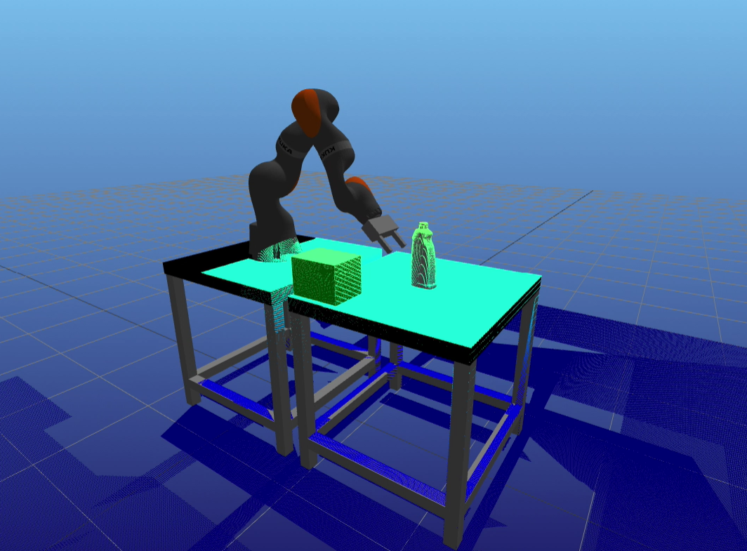
# Import stuff to be used in this notebook. Run this first!
%reload_ext autoreload
%autoreload 2
import matplotlib.pyplot as plt
from matplotlib import cm
import numpy as np
import meshcat
import meshcat.geometry as g

from iterative_closest_point import icp, make_meshcat_color_array
from point_cloud_processing import (VisualizeTransformedScenePointCloud,
                                    SegmentBottleZfilter,
                                    FindBottlePointInCroppedScenePointCloud,
                                    SegmentBox,
                                    GetBoxModelPointCloud)
# First start meshcat for visualization - this only has to be run once.

# If you interrupt the kernel of this notebook, you'll need to run this cell again to
# restart the meshcat server, and then refresh the visualization window.

# This will open a mesh-cat server in the background, click on the url to display visualization in a separate window.
vis = meshcat.Visualizer()
# Run this if you feel the visualizer is messed up and want to start over.
vis.delete()
0. Viewing the point cloud in meshcat
You are provided with a point cloud of the scene, which includes the tables, the bottle, the box and the robot at its upright posture. The coordinates of the points in the point cloud are expressed relative to the world frame W.
Run the following cell to take a look at the scene point cloud in meshcat. The color of the points are determined by their z-coordinates (blue: low, red: high). Note that there are a lot of points on the floor (shown in blue). In practice, these points are helpful to align point clouds generated by multiple cameras.
You will be asked to find
- the pose (position and orientation) of the bottle, and
- the pose of the green box.
# load scene point cloud
scene_point_cloud = np.load('./resources/scene_point_cloud.npy')

# color point cloud bazed on height (z)
min_height = scene_point_cloud[:,2].min()
max_height = scene_point_cloud[:,2].max()*1.1
colors = cm.jet((scene_point_cloud.T[2, :] - min_height) / (max_height - min_height)).T[0:3, :]

# show point cloud in meshcat
vis.delete()
vis["scene_point_cloud"].set_object(
    g.PointCloud(position=scene_point_cloud.T,
                 color=colors,
                 size=0.002))
1. Estimating the pose of the bottle in the world frame using ICP.
Let's first load the model point cloud. A red point cloud in the shape of the bottle will appear at the origin after running the cell below. Rotate the camera and zoom in to see it.
# Load point cloud of the bleach bottle.
bottle_point_cloud_model = np.load('./resources/bleach_bottle_point_cloud.npy')
n_model = bottle_point_cloud_model.shape[0]

# show point cloud in meshcat
vis['model_point_cloud'].set_object(
    g.PointCloud(bottle_point_cloud_model.T, make_meshcat_color_array(n_model, 0.5, 0, 0), size=0.002))
As the scene frame S is the same as the world frame W, if we can find the transform X_MS, then the pose of the model in the world frame can be found by inverting X_MS, i.e. X_WM = X_MS^(-1).
However, running ICP between model_point_cloud and scene_point_cloud probably won't give meaningful results, because the majority of the points in scene_point_cloud are outliers, e.g. table/box/ground points. For the fun of it, you can run the following cell to see what happens if we do that. It's gonna take a while because there are quite a few (1228800, to be exact) points in the scene point cloud.
# Call ICP to match full scene point cloud to model point cloud.
X_MS_bottle, mean_error, num_iters = \
    icp(scene_point_cloud, bottle_point_cloud_model, max_iterations=100, tolerance=1e-5)
print("X_MS_bottle:\n", X_MS_bottle.matrix())
print("mean error:", mean_error)
print("total iterations run:", num_iters)

# Create a yellow meshcat point cloud for visualization.
VisualizeTransformedScenePointCloud(X_MS_bottle, scene_point_cloud, vis)
A natural way to resolve this issue is to run ICP with only the scene points that correspond to the object of interest. The process of cropping out the correct subset of scene_point_cloud that corresponds to the model is known as segmentation, which is still an area of active research. Later in the course, we'll talk more about using other methods such as CNN to get initial estimates of object location and better segmentations. In this pset, however, we'll try segmentation with some heuristics.
The most straightforward heuristics is perhaps the "z-filter". Assuming that we know the height of the table, then every point with a z-coordinate smaller than that can be discarded. We've written a function that implements the z-filter for you:
from point_cloud_processing import table_top_z_in_world

# Segment bottle points from scene
scene_point_cloud_cropped = SegmentBottleZfilter(scene_point_cloud, z_threshold=table_top_z_in_world+0.001)

# Delete the messy yellow point cloud.
vis['transformed_scene'].delete()

# Replace the scene point cloud with the cropped version.
vis["scene_point_cloud"].set_object(
    g.PointCloud(position=scene_point_cloud_cropped.T,
                 color=make_meshcat_color_array(scene_point_cloud_cropped.shape[0], 0, 0.0, 1.0),
                 size=0.002))
You've probably noticed that there are more than one objects on the table. We need the bottle, but not the box or the bottom of the robot.
Your task is to complete function FindBottlePointInCroppedScenePointCloud in point_cloud_processing.py to create a segmentation that allows ICP to converge to the correct pose.
To segment the bottle from the z-filtered point cloud, you could use k-means, which is simple to implement or some variant of "connected components" as described [here] (https://cs.gmu.edu/~kosecka/ICRA2013/spme13_trevor.pdf). K-means should work in this case but would have trouble if the objects were more complicated or near to each other.
You can also assume we know that the bottle should be close to bottle_center_initial_guess = [0.8, 0, table_top_z_in_world] in world frame. The cluster whose mean is closest to that given point is the point cloud of the bottle.
from point_cloud_processing import bottle_center_initial_guess
indices_bottle = FindBottlePointInCroppedScenePointCloud(scene_point_cloud_cropped, bottle_center_initial_guess)

# Delete the messy yellow point cloud.
vis['transformed_scene'].delete()

# Replace scene point cloud with the segmented point cloud.
vis['scene_point_cloud'].set_object(
    g.PointCloud(scene_point_cloud_cropped[indices_bottle].T,
                 make_meshcat_color_array(len(indices_bottle), 0., 0., 1.0), size=0.002))
Running ICP on the segmented point cloud should give a much better estimation of the bottle's pose, but things could still go wrong... You can experiment with different intial guesses to see how it affect the estimated pose.
# Call ICP to match bottle_points to model point cloud
X_MS_bottle, mean_error, num_iters = \
    icp(scene_point_cloud_cropped[indices_bottle], bottle_point_cloud_model,
        init_guess = np.eye(4), max_iterations=100, tolerance=1e-8)
print("mean error:", mean_error)
print("total iterations run:", num_iters)

# compare ground truth of the bottle pose in world frame with the one returned by ICP
from point_cloud_processing import X_WObject
print("X_WBottle, ground truth:\n", X_WObject.matrix())
print("X_WBottle, estiated by ICP\n", X_MS_bottle.inverse().matrix())

# Display the transfomed scene points in yellow in meshcat.
VisualizeTransformedScenePointCloud(X_MS_bottle, scene_point_cloud_cropped[indices_bottle], vis)
2. Estimating the pose of the box in the world frame using ICP.
First, let's load the model points of the box. The model point cloud is generated by uniformly sampling points on the faces of the box.
num_points = 3000
box_point_cloud_model = GetBoxModelPointCloud(num_points=num_points)

# clear visualizer
vis.delete()

# show point cloud in meshcat
vis['model_point_cloud'].set_object(
    g.PointCloud(box_point_cloud_model.T, make_meshcat_color_array(num_points, 0.5, 0, 0), size=0.002))
We've done the segmentation for you this time.
# Segment box points from scene
box_point_cloud_scene = SegmentBox(scene_point_cloud)

# show point cloud in meshcat
vis["scene_point_cloud"].set_object(
    g.PointCloud(position=box_point_cloud_scene.T,
                 color=make_meshcat_color_array(box_point_cloud_scene.shape[0], 0, 0.5, 0),
                 size=0.002))
Notice that the segmented box does not have any points on its bottom face (because no camera can see it). Trying to run ICP between the point cloud of a bottomless box and a point cloud consisting of points uniformly sampled from the surface of the box would probably generate wrong results.
The following cell runs ICP on the box for 10 times. Every time, a new model point cloud is generated by randomly sampling a new set of points.
You can watch the estimated poses displayed in meshcat. We're trying to show how brittle ICP can be in this case: the success rate is only about 50% at its best, even though all sampled point clouds look similar.
X_WBox.translation()
# get ground truth box pose.
from point_cloud_processing import X_WBox

success_count = 0
for i in range(10):
    i += 1
    box_point_cloud_model = GetBoxModelPointCloud(num_points=3000)
    X_MS_box, mean_error, num_iters = \
        icp(box_point_cloud_scene, box_point_cloud_model,
            init_guess=np.eye(4), max_iterations=100, tolerance=1e-5)

    X_error = X_MS_box.multiply(X_WBox)
    is_rotation_close = np.abs(X_error.translation()).max() < 0.02
    is_position_close = X_error.rotation().ToQuaternion().w() > 0.99

    is_successful = is_position_close and is_rotation_close
    if is_successful:
        success_count += 1

    print("trial ", i, 'success' if is_successful else 'fail')

    # Create a yellow meshcat point cloud for visualization.
    VisualizeTransformedScenePointCloud(X_MS_box, box_point_cloud_scene, vis)

print("success_count:", success_count)
Why does ICP work unreliably in this case? First of all, the scene point cloud is incomplete: it doesn't have a bottom face. In addition, due to the positioning of cameras, the distribution of points on different faces of the scene point cloud is not uniform: there are a lot more points on the top face.
As discussed in the lectures, you could try normal ICP, or formulating pose estimation as an inverse kinematics problem with constraints. Fill in function EstimateBoxPoseSmartly in point_cloud_processing.py with your improved strategy.
This task is optional. Bonus points will be given if your strategy can succeed more than 8 out of 10 times.
Run Tests
Running the cell below will print out a score for every test and the total score.
import subprocess
# Run the tests
subprocess.run("python3 ./test_pset_2.py test_results.json", shell=True)

import test_pset_2
# Print the results json for review
print(test_pset_2.pretty_format_json_results("test_results.json"))