Pset #3 part 1 of 2: pick and place using the iiwa arm
In this notebook, you'll be asked to use IK (inverse kinematics) and to plan trajectories that pick up an object and place it at a designated location. To get a quick idea of what needs to be accomplished, click on the picture below to watch the full task.
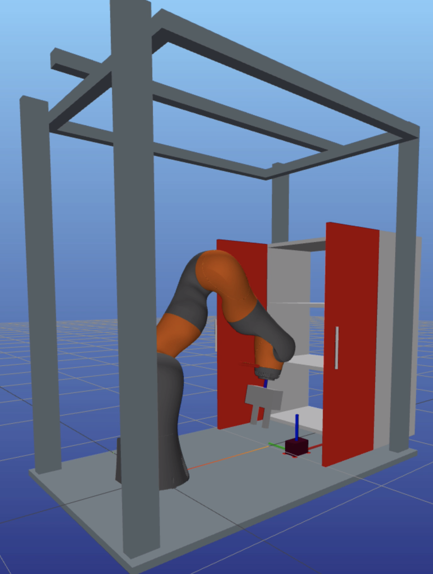
The manipulation station you will be working with in the labs. Also shown in the video are the body frames of the object and link 7 (the last link of the robot, which plays a similar role as link ee in pset 1). Red bars indicate contact forces.
0. Setup
# Import stuff to be used in this notebook. Run this first!
%reload_ext autoreload
%autoreload 2
import matplotlib.pyplot as plt
from matplotlib import cm
import numpy as np
import meshcat
import meshcat.geometry as g
from manip_station_sim.plan_utils import PlotJointLog, PlotIiwaPositionLog
# First start meshcat for visualization - this only has to be run once.

# If you interrupt the kernel of this notebook, you'll need to run this cell again to
# restart the meshcat server, and then refresh the visualization window.

# This will open a mesh-cat server in the background,
# click on the url to display visualization in a separate window.
vis = meshcat.Visualizer()
# Run this if you feel the visualizer is messed up and want to start over.
vis.delete()
Run this cell and observe what the robot does in meshcat.
from manip_station_sim.manipulation_station_simulator import ManipulationStationSimulator
from manip_station_sim.robot_plans import JointSpacePlan
from iiwa_pick_and_place_trajectory_generation import GenerateIiwaTrajectoriesAndGripperSetPoints
from test_pset_3 import X_WO, q0

# Construct simulator.
sim = ManipulationStationSimulator(X_WO)

# Create Plans
q_traj_list, gripper_setpoint_list = GenerateIiwaTrajectoriesAndGripperSetPoints(X_WO)
plan_list = [JointSpacePlan(q_traj) for q_traj in q_traj_list]

# real_time_rate=0 means running the simulation as fast as possible.
# Setting real_time_rate 1 to run the simulation close to real time.
(iiwa_position_command_log, iiwa_position_measured_log,
    iiwa_external_torque_log, iiwa_velocity_estimated_log,
    plant_state_log, t_plan) = sim.RunSimulation(
    q0, plan_list, gripper_setpoint_list, extra_time=2.0, real_time_rate=1.0)
# Plot joint velocity
PlotJointLog(iiwa_velocity_estimated_log, legend="qDt", y_label="rad/s")
# Plot joint torque
PlotJointLog(iiwa_external_torque_log, legend="tau_ext", y_label="N*m")
# Plot joint position logs.
PlotIiwaPositionLog(iiwa_position_command_log, iiwa_position_measured_log)
1. Trajectory planning task
Let's define a few things before laying out the requirements.
- Q is a point fixed to the end effector frame.
p_L7Q = [0, 0, 0.21]is the coordinates of pointQin frameL7expressed inL7, whereL7is the body frame of link 7 of the robot (the last link).p_WQ, whereWis the world frame andQrepresents point Q, denotes the coordinates of Q in frameW.
Executing trajectories provided to you in function GenerateIiwaTrajectoriesAndGripperSetPoints (in file iiwa_pick_and_place_trajectory_generation.py), you'll find that robot arm
- starts at
q0, which is imported fromtest_pset_3.py, - goes to
q_home, which is defined at the beginning ofiiwa_pick_and_place_trajectory_generation.py, - moves point Q to
p_WQ_home = [0.5, 0, 0.4]and stays there, and finally - opens the gripper.
You might have noticed that the trajectory from q0 to q_home is not in the list of trajectories returned by GenerateIiwaTrajectoriesAndGripperSetPoints. Indeed, it is a safety feature we have implemented, such that if the current robot joint space position is too far away from the commanded position at the beginning of your trajectories, the robot will follow a joint-space cubic spline to transition smoothly to the beginning of your trajectories.
Your ask is to pick up from where the robot stops. Complete function GenerateIiwaTrajectoriesAndGripperSetPoints. The completed function should return a list (python list) of trajectories (pydrake.trajectories.PiecewisePolynomial) that picks up the foam brick and places it on the middle shelf of the cabinet.
Each trajectory has a duration that the simulator is aware of. The simulator makes sure that all trajectories are executed, and simulates for an additional 2 seconds for velocities to damp out. At the end of the simulation, your system (robot + gripper + foam brick) needs to satisfy the following requirements:
- the robot returns to
q_home; - everything should be have close-to-zero velocity (doesn't look like it's moving in the visualizer);
- the foam brick is on the middle shelf of the cabinet;
In addition, throughout the simulation, the joint torque of any of the robots' joints cannot exceed $30 \;\mathrm{N} \cdot \mathrm{m}$, and the angular velocity of any of the joints cannot exceed $0.5 \; \mathrm{rad/s}$.
The gripper fingers and body are connected by translational joints. Setting gripper_setpoint to 0.1 (meters) means the gripper is open, setting it to 0.01 to close the gripper.
Hints and tips
Drake utilities that will probably come in handy
- You'll probably make heavy use of
pydrake.trajectories.PiecewisePolynomial. The C++ documentation can be found here. Examples on how to use the python bindings can be found here. pydrake.mathhas convenient methods for the creation and conversion of converting rotation representations. For example, you've seenpydrake.math.RotationMatrixandpydrake.math.RollPitchYaw. Although these docs are written for C++, the python bindings share very similar function signatures as their C++ counter part. If you find the python documentation a bit confusing, the doxygen documentation could be helpful.
Task space interpolation with IK
Solving IK gives you points in the robot's joint space. Interpolating between points that are "far away" in joint space could create unexpected end effector trajectories in task space. This could lead to undesirable results such as collision.
To make sure that end effector moves more or less along a straight line in task space, we recommend you implement the following method.
def MoveEndEffectorAlongStraightLine(
    p_WQ_start, p_WQ_end, duration, get_orientation, q_initial_guess, num_knots):
    """
    THIS IS PSEUDO CODE!
    p_WQ_start is the starting position of point Q (the point Q we defined earlier!)
    p_WQ_end is the end position of point Q.
    duration is the duration of the trajectory measured in seconds.
    get_orientation(i, n) is a function that returns the interpolated orientation R_WL7 at the i-th knot point out of n knot points. It can simply return a constant orientation, but changing the orientation of link 7 should be helpful for placing the object on the shelf.
    num_knots is the number of knot points in the trajectory. Generally speaking,the larger num_knots is, the smoother the trajectory, but solving for more knot points also takes longer. You can start by setting num_knots to 10, which should be sufficient for the task.
    """
    t_knots = np.linspace(0, duration, num_knots+1)
    q_knots = np.zeros((num_knots, plant.num_positions()))
    q_knots[0] = q_initial_guess

    for i in range(num_knots):
        ik = pydrake.multibody.inverse_kinematics.InverseKinematics(plant)
        ik.AddPositionConstraint(...) # interpolate between p_WQ_start and p_WQ_end
        ik.AddOrientationConstraint(...) # call get_orientation(i, num_knots).
        if i == 0:
            ik.SetInitialGuess(q_initial_guess)
        else:
            # This is very important for the smoothness of the whole trajectory.
            ik.SetInitialGuess(q_knots[i - 1])
        result = pydrake.solvers.mathematicalprogram.Solve(ik.prog())
        assert result.get_solution_result() == SolutionResult.kSolutionFound
        q_knots[i] = result.GetSolution(ik.q())

    return PiecewisePolynomia.Cubic(q_knots) # return a cubic spline that connects all q_knots.
An important detail is that the initial guess for the (i+1)-th IK should be the solution to the i-th IK, which significantly improves the overall smoothness of the trajectory.
# utility: draw a frame at pose X_WC.
from pydrake.systems.meshcat_visualizer import AddTriad
from pydrake.math import RigidTransform
X_WC = RigidTransform()
X_WC.set_translation([1.1, 0., 0.55])
AddTriad(vis, "test", "tests", length=0.15, radius=0.006)
vis["tests"]["test"].set_transform(X_WC.matrix())
Run Tests
Running the cell below will print out a score for every test and the total score.
import subprocess
# Run the tests
subprocess.run("python3 ./test_pset_3.py test_results.json", shell=True)

import test_pset_3
# Print the results json for review
print(test_pset_3.pretty_format_json_results("test_results.json"))