Problem Set #5 part 2: controllers that open cupboard doors¶

In this notebook, we will take a more careful look at controllers, which have been treated as a black box that generates torques ($\tau_{\text{cmd}}$) to drive the robot to desired configurations ($q_{\text{ref}}$).

1. Rigid body dynamics¶

Almost every controller starts with writing down the equations of motion ($F=ma$) of the robot: \begin{equation} M(q)\ddot{q} + C(q, \dot{q}) + g(q) = \tau_{m} + \tau_{external} \quad\quad\quad (1) \end{equation}

$q \in \mathbb{R}^7$ is the configuration, or joint angles of the iiwa arm.
$\dot{q}, \ddot{q} \in \mathbb{R}^7$ are the generalized velocities and accelerations.
$M(q) \in \mathbb{R}^{7\times 7}$ is the mass matrix, which depends on $q$.
$C(q, \dot{q}) \in \mathbb{R}^7$ is the Coriolis forces.
$g(q) \in \mathbb{R}^7$ is the torque (generalized forces) generated by gravity.
$\tau_{external}$ is the torque generated by external contact. It is zero if the robot is not making contact with the environment.
$\tau_{m}$ is the torque applied to the robot by the robot's motors.

2. Robot controller and closed-loop dynamics¶

The controller of many industrial robotic arms can be decomposed into two layers: an inner, fast loop which directly controls motor torque (shown as "robot controller" in the figure below); and an outer, slower loop which accepts commands from users (shown as "your controller").

Figure: Schematic diagram of frames and points in `ManipulationStation`. Frames are drawn in 2D for simplicity.

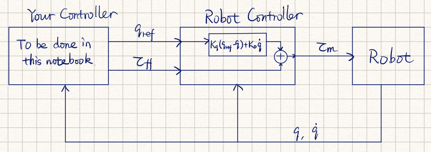
As a result of this decomposition, direct control of motor torque is usually not available through industrial robotic arms' API. As an example, the kuka iiwa robots used in lab sessions only accept a iiwa_position_command($q_{ref}$) and a iiwa_feedforward_torque_command ($\tau_{ff}$). The robot controller takes command from the user controller and computes the motor torque $\tau_m$ using \begin{align} \tau_{m} &= K_q(q_{ref} - q) - D_q\dot{q} + g(q) + \tau_{\text{ff}} \end{align} where $K_q$ and $D_q$ are diagonal gain matrices. This inner loop controller gives the following closed-loop dynamics: \begin{align} M(q) \ddot{q} + \left(C(q, \dot{q}) + D_q\right)\dot{q} + K\left( q - q_{ref}\right) = \tau_{external} + \tau_{\text{ff}} \end{align}

3. Tasks¶

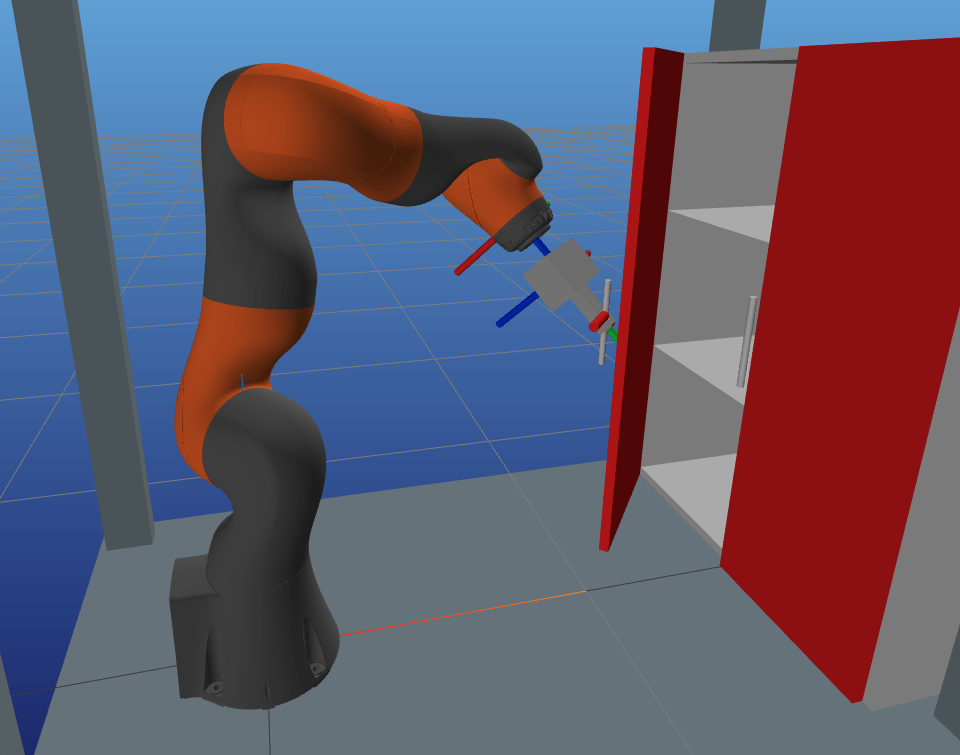
Previously you have done various tasks by repeatedly solving inverse kinematics. This time around, we'll be comparing IK with Jacobian-based controllers . Specifically, you'll be asked to open the left door of the cupboard in ManipulationStation by mapping velocities or Cartesian forces into joint torques with the help of Jacobians. As usual, there is a Youtube video that shows what needs to be done. Click on the figure below to watch it.

Video: opening the left door with impedance control.

4. Geometry of `ManipulationStation`¶

Figure: Schematic diagram of frames and points in `ManipulationStation`. Frames are drawn in 2D for simplicity.

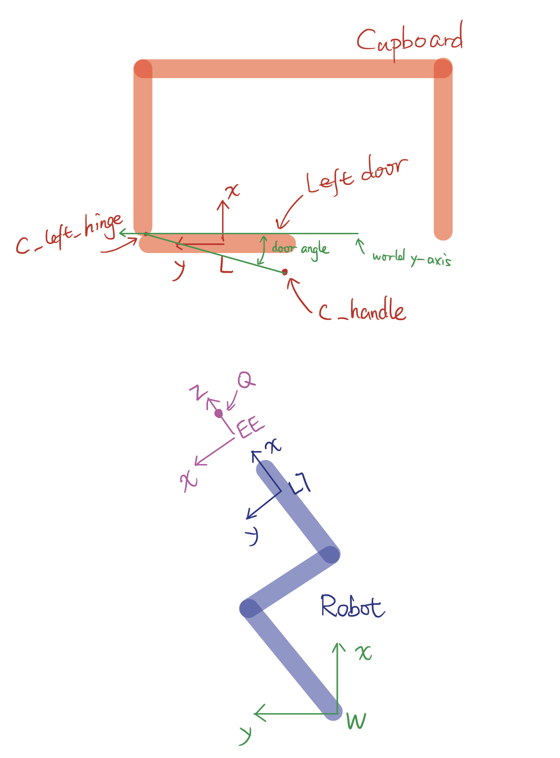
W: world frame.
L: frame fixed to the cupboard left door.
C_left_hinge: the center of the hinge relative to frame L.
C_handle: the center of the door handle relative to frame L.
L7: frame fixed to link 7 (last link) of the robot.
EE: frame fixed to the end effector of the robot, which is also fixed w.r.t. L7.
Q: a point fixed in frame EE (and L7).

5. Geometric Jacobian¶

In Drake's notation convention, geometric Jacobians are denoted by $J_v$. They map the robot's joint velocity $\dot{q}$ to the angular velocity of a frame, and the Cartesian velocity of a point fixed to that frame. The tasks in this notebook are centered around using geometric Jacobians to map quantities between joint and Cartesian spaces.

To open the door, the robot interacts with the door handle at a point Q fixed in frame L7. As $J_v$ is by definition a mapping from joint to Cartesian velocities, the following equality holds: \begin{equation} \begin{pmatrix} [^W\omega^{L7}]_W\\ [^W v_Q]_W \end{pmatrix} \quad =\quad [^W{J_v}^{L7}_Q]_W \quad \dot{q} \end{equation}

$[^W\omega^{L7}]_W$ is the angular velocity of frame L7 relative to frame W, expressed in frame W.
$[^W v_Q]_W$ is the linear velocity of point Q (which is fixed in L7), expressed in frame W.
$[^W{J_v}^{L7}_Q]_W \in \mathbb{R}^{6 \times 7}$ (written as Jv_WL7q in code) is the geometric Jacobian of point Q which is fixed in frame L7, relative to frame W and expressed in frame W.

In addition, the transpose of geometric Jacobians maps Cartesian forces/torques back to joint torque: \begin{align} [F^{L7}]_W \quad &=\quad \begin{pmatrix} [\tau^{L7}]_W\\ [f^Q]_W \end{pmatrix}\\ \tau \quad &=\quad {[^W{J_v}^{L7}_Q]_W}^{\intercal} \quad [F^{L7}]_W \end{align}

$[F^{L7}]_{W} \in \mathbb{R}^6$ is the spatial force on body(frame) L7.
$[m^{L7}]_W \in \mathbb{R}^3$ is the moment on body L7.
$[f^Q]_W \in \mathbb{R}^3$ is the force at point Q, which is fixed to body L7.

Setup¶

# Import stuff to be used in this notebook. Run this first!
%reload_ext autoreload
%matplotlib notebook
%autoreload 2

import matplotlib.pyplot as plt
from matplotlib import cm
import numpy as np
import meshcat
import meshcat.geometry as g
from manip_station_sim.plan_utils import PlotJointLog, PlotIiwaPositionLog

from pydrake.math import RollPitchYaw, RotationMatrix
from pydrake.trajectories import PiecewisePolynomial

# duration of the door-opening trajectory/plan.
duration_arc = 10

# First start meshcat for visualization - this only has to be run once.

# If you interrupt the kernel of this notebook, you'll need to run this cell again to 
# restart the meshcat server, and then refresh the visualization window. 

# This will open a mesh-cat server in the background, 
# click on the url to display visualization in a separate window. 
vis = meshcat.Visualizer()

# Run this if you feel the visualizer is messed up and want to start over.
vis.delete()

Task 1. Arc tracking and door opening by IK¶

Perhaps the most straightforward solution to open the door is to solve IK at a few knot points along the arc of the door handle and interpolate between the solutions using a cubic polynomial.

Your task is to complete InverseKinPointwise in ./manip_station_sim/ik_utils.py. This function is very similar to MoveEndEffectorAlongStraightLine in Pset 3a. The difference is that InverseKinPointwise supports interpolating along user-defined trajectories, including arcs. The functions which compute reference position for Q and reference orientation for L7 have been provided for you in open_left_door.py.

You can simulate with the doors open or closed by toggling the initial condition for door angles.

from manip_station_sim.manipulation_station_simulator import ManipulationStationSimulator
from manip_station_sim.robot_plans import JointSpacePlan
from pydrake.trajectories import PiecewisePolynomial
from open_left_door import InterpolateArc, InterpolateYawAngle, p_L7Q, q_home, q0
from ik_utils import InverseKinPointwise

# Generate plan list
# follow arc
qtraj_open_door, q_knots = InverseKinPointwise(
                    InterpolatePosition=InterpolateArc,
                    InterpolateOrientation=InterpolateYawAngle,
                    p_L7Q=p_L7Q,
                    duration=duration_arc,
                    num_knot_points=10,
                    q_initial_guess=q_home,
                    position_tolerance=0.001)

# close gripper
q_knots_close_gripper = np.zeros((2, 7))
q_knots_close_gripper[0] = q_knots[0]
qtraj_close_gripper = PiecewisePolynomial.ZeroOrderHold(
                            [0, 1], q_knots_close_gripper.T)

plan_list = [JointSpacePlan(qtraj) for qtraj in [qtraj_close_gripper, qtraj_open_door]]
gripper_setpoint_list = [0.005, 0.005]

# Simulate with doors closed
# door_angles = np.array([-0.001, 0.001])

# Simulate with doors open
door_angle = np.pi/2 - 0.001
door_angles = np.array([-door_angle, door_angle])

# Construct simulator.
sim = ManipulationStationSimulator()

# real_time_rate=0 means running the simulation as fast as possible. 
# Setting real_time_rate 1 to run the simulation close to real time.
(iiwa_position_command_log, iiwa_position_measured_log,
    iiwa_external_torque_log, iiwa_velocity_estimated_log,
    plant_state_log, t_plan) = sim.RunSimulation(
    q_home, door_angles, plan_list, gripper_setpoint_list, extra_time=2.0, real_time_rate=0.0)

The cells below generate plots for tracking performance evaluation.

(2 points) answer the following questions. Include your answers and relevant plots in a PDF file.

With the doors open, generate tracking error plots for trajectories with 2, 5 and 10 knot points. How does the number of knot points affect tracking error?
Zoom in to the xy position plot of Q. Is the magnitude of tracking error consistent along the arc with the doors open? Why do you think the error is (in)consistent? What happens if the doors are closed?

# Compute position of Q from simulation logs.
from manip_station_sim.plan_utils import CalcQPositionInWorldFrame, CalcL7PoseInWolrdFrame
from open_left_door import p_L7Q, p_WC_left_hinge, CalcHandleArcPoints, r_handle

# Get the section of the trajectory related to arc-tracking.
t_start = 11
t_end = 11 + duration_arc
n_start = int(t_start / 0.01)
n_end = int(t_end / 0.01) + 1

list_X_WL7, t = CalcL7PoseInWolrdFrame(iiwa_position_command_log, n_start=n_start, n_end=n_end)
p_WQ = CalcQPositionInWorldFrame(list_X_WL7, p_L7Q)

# points on the arc
points_on_handle_arc = CalcHandleArcPoints()

# Plot radial tracking error, which measures how much the trajectory of Q deviates from the door arc.
from open_left_door import CalcRadialTrackingError
r_error = CalcRadialTrackingError(p_WQ)

fig = plt.figure(dpi = 100)
plt.plot(t, r_error)
ax = plt.gca()
ax.grid(True)
ax.set_xlabel('time (s)')
ax.set_ylabel('r_tracking_error (m)')
plt.title("radial tracking error")
plt.show()

# Plot orientation tracking error.
from open_left_door import CalcOrientationTrackingError
angle_error_list = CalcOrientationTrackingError(list_X_WL7, t, duration_arc)

fig = plt.figure(dpi=100)
plt.plot(t, angle_error_list)
ax = plt.gca()
ax.grid(True)
ax.set_xlabel('time (s)')
ax.set_ylabel('error angle (rad)')
plt.title("Orientation tracking error")
plt.show()

# Plot position of Q in the xy-plane of world frame.
fig = plt.figure(figsize=(5, 5), dpi=120)
ax = plt.gca()
ax.plot(points_on_handle_arc[:, 0], 
        points_on_handle_arc[:, 1],
        linewidth=2,
        label="handle arc")
ax.plot(p_WQ[:, 0], 
        p_WQ[:, 1], linewidth=1.5,
        label="Q path")
ax.plot(p_WC_left_hinge[0], p_WC_left_hinge[1], "*", 
           label="door hinge", markersize=20)

ax.set_aspect('equal', 'box')
ax.set_xlabel('x_world (m)')
ax.set_ylabel('y_world (m)')
ax.grid(True)
ax.set_title('position of Q in the xy-plane of world frame')
ax.legend()
plt.show()

Task 2: Arc tracking and door opening by mapping velocities.¶

This controller uses the Jacobian to compute desired joint velocities: \begin{align} V_{\text{des}} &= \begin{pmatrix} K_{\omega} \theta \pmb{n} \\ K_v e_{xyz} \end{pmatrix}\\ \dot{q}_{des} &= {[^W{J_v}^{L7}_Q]_W}^{+} V_{\text{des}} \\ q_{ref} &= q_{current} + \dot{q}_{des} \Delta t \\ \tau_{\text{ff}} &= 0 \end{align}

$e_{xyz} = [p_Q^W]_{W, \text{ref}} - [p_Q^W]_{W}$ is the position tracking error of point Q.
$\theta$ and $\pmb{n}$ are the angle and axis of the orientation error $\mathbf{R}^{L7}_{L7_r}$. Computation of position and orientation errors have been implemented for you in IiwaTaskSpacePlan.CalcPositionError and IiwaTaskSpacePlan.CalcOrientationError.
${[^W{J_v}^{L7}_Q]_W}^{+}$ is the pseudo inverse of $[^W{J_v}^{L7}_Q]_W$
$\Delta t$ is the controller time step, which is the control_period argument in the function you need to complete.
$K_v$ and $K_\omega$ are 3x3 diagonal gain matrices. $K_v = \text{diag}([100, 100, 100])$ and $K_v = \text{diag}([50, 50, 50])$ have been working well in our tests.

Complete calc_p_Q, calc_R_WL7_ref and IiwaTaskSpaceVelocityPlan.CalcPositionCommand in robot_plan.py with the controller described above.

from manip_station_sim.manipulation_station_simulator import ManipulationStationSimulator
from manip_station_sim.robot_plans import JointSpacePlan, IiwaTaskSpaceVelocityPlan
from ik_utils import SolveOneShotIk
from open_left_door import p_WC_handle, p_L7Q, q_home, theta0_hinge, calc_p_Q, calc_R_WL7_ref

# Generate plan list
R_WL7_0 = RollPitchYaw(0, np.pi/4*3, 0).ToRotationMatrix()
q_start = SolveOneShotIk(
            p_WQ_ref=p_WC_handle,
            R_WL7_ref=R_WL7_0,
            p_L7Q=p_L7Q,
            q_initial_guess=q_home,
            position_tolerance=0.0005)

# close gripper
q_knots = np.zeros((2, 7))
q_knots[0] = q_start
qtraj_close_gripper = PiecewisePolynomial.ZeroOrderHold([0, 1], q_knots.T)

# open door using task space plan
task_space_plan = IiwaTaskSpaceVelocityPlan(
    calc_p_Q=calc_p_Q,
    calc_R_WL7_ref=calc_R_WL7_ref,
    duration=duration_arc,
    p_L7Q=p_L7Q)

plan_list = [JointSpacePlan(qtraj_close_gripper), task_space_plan]
gripper_setpoint_list = [0.005, 0.005]

# Simulate with doors closed
# door_angles = np.array([-0.001, 0.001])

# Simulate with doors open
door_angle = np.pi/2 - 0.001
door_angles = np.array([-door_angle, door_angle])

# Construct simulator.
sim = ManipulationStationSimulator()

# real_time_rate=0 means running the simulation as fast as possible. 
# Setting real_time_rate 1 to run the simulation close to real time.
(iiwa_position_command_log, iiwa_position_measured_log,
    iiwa_external_torque_log, iiwa_velocity_estimated_log,
    plant_state_log, t_plan) = sim.RunSimulation(
    q_home, door_angles, plan_list, gripper_setpoint_list, extra_time=2.0, real_time_rate=0.0)

(2 points) answer the following questions. Include your answers and relevant plots in a PDF file.

Generate tracking error plots with the doors open. How does the tracking error compare with the trajectory generated from IK? (Hint: tracking error should be smaller)
Zoom in to the xy position plot of Q. Is the magnitude of tracking error consistent along the arc with the doors open? Why do you think the error is (in)consistent? What happens if the doors are closed? (Hint: error along the arc should be smaller and more consistent).

# Compute position of Q from simulation logs.
from manip_station_sim.plan_utils import CalcQPositionInWorldFrame, CalcL7PoseInWolrdFrame
from open_left_door import p_L7Q, p_WC_left_hinge, CalcHandleArcPoints, r_handle

# Get the section of the trajectory related to arc-tracking.
t_start = 11
t_end = 11 + duration_arc
n_start = int(t_start / 0.01)
n_end = int(t_end / 0.01) + 1

list_X_WL7, t = CalcL7PoseInWolrdFrame(iiwa_position_command_log, n_start=n_start, n_end=n_end)
p_WQ = CalcQPositionInWorldFrame(list_X_WL7, p_L7Q)

# points on the arc
points_on_handle_arc = CalcHandleArcPoints()

# Plot Radial tracking error.
from open_left_door import CalcRadialTrackingError
r_error = CalcRadialTrackingError(p_WQ)

fig = plt.figure(dpi = 100)
plt.plot(t, r_error)
ax = plt.gca()
ax.grid(True)
ax.set_xlabel('time (s)')
ax.set_ylabel('r_tracking_error (m)')
plt.title("radial tracking error")
plt.show()

# Plot orientation tracking error.
from open_left_door import CalcOrientationTrackingError
angle_error_list = CalcOrientationTrackingError(list_X_WL7, t, duration_arc)

fig = plt.figure(dpi=100)
plt.plot(t, angle_error_list)
ax = plt.gca()
ax.grid(True)
ax.set_xlabel('time (s)')
ax.set_ylabel('error angle (rad)')
plt.title("Orientation tracking error")
plt.show()

# Plot position of Q in the xy-plane of world frame.
fig = plt.figure(figsize=(5, 5), dpi=120)
ax = plt.gca()
ax.plot(points_on_handle_arc[:, 0], 
        points_on_handle_arc[:, 1],
        linewidth=2,
        label="handle arc")
ax.plot(p_WQ[:, 0], 
        p_WQ[:, 1], linewidth=1.5,
        label="Q path")
ax.plot(p_WC_left_hinge[0], p_WC_left_hinge[1], "*", 
           label="door hinge", markersize=20)

ax.set_aspect('equal', 'box')
ax.set_xlabel('x_world (m)')
ax.set_ylabel('y_world (m)')
ax.grid(True)
ax.set_title('position of Q in the xy-plane of world frame')
ax.legend()
plt.show()

Task 3: Arc tracking and door opening by mapping forces.¶

It is also possible to send feedforward torque command, and bypass the position command by sending the current position of the robot as position command: \begin{align} F &= \begin{pmatrix} K_{\omega} \theta \pmb{n} \\ K_v e_{xyz} \end{pmatrix}\\ \tau_{\text{ff}} &= {[^W{J_v}^{L7}_Q]_W}^{\intercal} F \\ q_{ref} &= q_{current} \end{align}

Complete IiwaTaskSpaceImpedancePlan.CalcTorqueCommand in robot_plan.py with the controller described above.

from manip_station_sim.manipulation_station_simulator import ManipulationStationSimulator
from manip_station_sim.robot_plans import JointSpacePlan, IiwaTaskSpaceImpedancePlan
from ik_utils import SolveOneShotIk
from open_left_door import p_WC_handle, p_L7Q, q_home, theta0_hinge, calc_p_Q, calc_R_WL7_ref

# Generate plan list
R_WL7_0 = RollPitchYaw(0, np.pi/4*3, 0).ToRotationMatrix()
q_start = SolveOneShotIk(
            p_WQ_ref=p_WC_handle,
            R_WL7_ref=R_WL7_0,
            p_L7Q=p_L7Q,
            q_initial_guess=q_home,
            position_tolerance=0.0005)

# close gripper
q_knots = np.zeros((2, 7))
q_knots[0] = q_start
qtraj_close_gripper = PiecewisePolynomial.ZeroOrderHold([0, 1], q_knots.T)

# open door using task space plan
task_space_plan = IiwaTaskSpaceImpedancePlan(
    calc_p_Q=calc_p_Q,
    calc_R_WL7_ref=calc_R_WL7_ref,
    duration=duration_arc,
    p_L7Q=p_L7Q)

plan_list = [JointSpacePlan(qtraj_close_gripper), task_space_plan]
gripper_setpoint_list = [0.005, 0.005]

# Simulate with doors closed
door_angles = np.array([-0.001, 0.001])

# Simulate with doors open
# door_angle = np.pi/2 - 0.001
# door_angles = np.array([-door_angle, door_angle])

# Construct simulator.
sim = ManipulationStationSimulator()

# real_time_rate=0 means running the simulation as fast as possible. 
# Setting real_time_rate 1 to run the simulation close to real time.
(iiwa_position_command_log, iiwa_position_measured_log,
    iiwa_external_torque_log, iiwa_velocity_estimated_log,
    plant_state_log, t_plan) = sim.RunSimulation(
    q_home, door_angles, plan_list, gripper_setpoint_list, extra_time=2.0, real_time_rate=0.0)

(2 points) answer the following questions. Include your answers and relevant plots in a PDF file.

Generate tracking error plots with the doors open. How does the tracking error compare with the other approaches?
Generate tracking error plots with the doors closed. How does closing the door affect tracking error?

# Compute position of Q from simulation logs.
from manip_station_sim.plan_utils import CalcQPositionInWorldFrame, CalcL7PoseInWolrdFrame
from open_left_door import p_L7Q, p_WC_left_hinge, CalcHandleArcPoints, r_handle

# Get the section of the trajectory related to arc-tracking.
t_start = 11
t_end = 11 + duration_arc
n_start = int(t_start / 0.01)
n_end = int(t_end / 0.01) + 1

list_X_WL7, t = CalcL7PoseInWolrdFrame(iiwa_position_command_log, n_start=n_start, n_end=n_end)
p_WQ = CalcQPositionInWorldFrame(list_X_WL7, p_L7Q)

# points on the arc
points_on_handle_arc = CalcHandleArcPoints()

# Plot Radial tracking error.
from open_left_door import CalcRadialTrackingError
r_error = CalcRadialTrackingError(p_WQ)

fig = plt.figure(dpi = 100)
plt.plot(t, r_error)
ax = plt.gca()
ax.grid(True)
ax.set_xlabel('time (s)')
ax.set_ylabel('r_tracking_error (m)')
plt.title("radial tracking error")
plt.show()

# Plot orientation tracking error.
from open_left_door import CalcOrientationTrackingError
angle_error_list = CalcOrientationTrackingError(list_X_WL7, t, duration_arc)

fig = plt.figure(dpi=100)
plt.plot(t, angle_error_list)
ax = plt.gca()
ax.grid(True)
ax.set_xlabel('time (s)')
ax.set_ylabel('error angle (rad)')
plt.title("Orientation tracking error")
plt.show()

# Plot position of Q in the xy-plane of world frame.
fig = plt.figure(figsize=(5, 5), dpi=120)
ax = plt.gca()
ax.plot(points_on_handle_arc[:, 0], 
        points_on_handle_arc[:, 1],
        linewidth=2,
        label="handle arc")
ax.plot(p_WQ[:, 0], 
        p_WQ[:, 1], linewidth=1.5,
        label="Q path")
ax.plot(p_WC_left_hinge[0], p_WC_left_hinge[1], "*", 
           label="door hinge", markersize=20)

ax.set_aspect('equal', 'box')
ax.set_xlabel('x_world (m)')
ax.set_ylabel('y_world (m)')
ax.grid(True)
ax.set_title('position of Q in the xy-plane of world frame')
ax.legend()
plt.show()

Utility functions¶

# Plot joint velocity
PlotJointLog(iiwa_velocity_estimated_log, legend="qDt", y_label="rad/s")

# Plot joint torque
PlotJointLog(iiwa_external_torque_log, legend="tau_ext", y_label="N*m")

# Plot joint position logs.
PlotIiwaPositionLog(iiwa_position_command_log, iiwa_position_measured_log)

Run Tests¶

Running the cell below will print out a score for every test and the total score.

import subprocess
# Run the tests
subprocess.run("python3 ./test_pset_5a.py test_results.json", shell=True)

import test_pset_5a
# Print the results json for review
print(test_pset_5a.pretty_format_json_results("test_results.json"))

Problem Set #5 part 2: controllers that open cupboard doors¶

1. Rigid body dynamics¶

2. Robot controller and closed-loop dynamics¶

3. Tasks¶

4. Geometry of ManipulationStation¶

5. Geometric Jacobian¶

Setup¶

Task 1. Arc tracking and door opening by IK¶

Task 2: Arc tracking and door opening by mapping velocities.¶

Task 3: Arc tracking and door opening by mapping forces.¶

Utility functions¶

Run Tests¶

4. Geometry of `ManipulationStation`¶