Problem Set #5 Part 1: Quaternions and rotations
In many branches of computer science (robotics included), unit quaternions are the preferred way of representing rotations in $\mathbb{R}^3$. In this notebook, we will explore some useful properties of quaternions and how they can be applied to the interpolation and control of rotations.
If you are not familiar with quaternions, you can read Section 1-4 of this tutorial [Jia2019] for more complete discussions on the topics covered in this notebook.
Setup
%reload_ext autoreload
%matplotlib notebook
%autoreload 2
import time

import numpy as np
import matplotlib.pyplot as plt
import meshcat

from pydrake.common.eigen_geometry import Quaternion
from pydrake.systems.meshcat_visualizer import AddTriad
from pydrake.math import RotationMatrix, RollPitchYaw, RigidTransform
# First start meshcat for visualization - this only has to be run once.

# If you interrupt the kernel of this notebook, you'll need to run this cell again to
# restart the meshcat server, and then refresh the visualization window.

# This will open a mesh-cat server in the background, click on the url to display visualization in a separate window.
vis = meshcat.Visualizer()
# Clear visualizer.
vis.delete()
Motivation: Interpolating Euler angles is a bad idea...
Running the cell below visualizes the interpolation between two rotations parametrized by Euler angles. The starting frame $A$ is shown as solid, and the end frame $B$ as translucent with a larger radius. Starting from frame $A$, you can see that the interpolated frames take some peculiar detours before arriving at frame $B$.
rpy_WA = np.array([-np.pi/4, 0, np.pi])
rpy_WB = np.array([np.pi, -np.pi/2, -np.pi/4])
R_WA = RollPitchYaw(rpy_WA).ToRotationMatrix()
R_WB = RollPitchYaw(rpy_WB).ToRotationMatrix()

# show path
vis.delete()
n = 70
for i in range(n):
    name = str(i)
    prefix = "euler_angles"
    radius = 0.005
    opacity = 0.3
    if i == 0:
        radius = 0.01
        opacity = 1
    elif i == n-1:
        radius = 0.03
        opacity = 0.5
    AddTriad(vis, name, prefix, radius=radius, opacity=opacity)
    rpy = rpy_WA + (rpy_WB - rpy_WA) / (n - 1) * i

    T = RigidTransform(RollPitchYaw(rpy).ToRotationMatrix(), np.zeros(3))
    vis[prefix][name].set_transform(T.matrix())

    # show interpolation over 10 seconds.
    time.sleep(10 / n)
1. Unit quaternions
A quaternion, customarily denoted by $q$, is a 4-tuple of real numbers. It can be decomposed into a scalar component $q_0 \in \mathbb{R}$ and a vector component $\pmb{q} \in \mathbb{R}^3$, i.e. \begin{equation} q = \left(q_0, \pmb{q} \right) = \left(q_0, \left(q_i, q_j, q_k\right) \right) \end{equation}
A unit quaternion is a quaternion with unit norm ($\|q\|^2=q_0^2 + \|\pmb{q}\|^2 = 1$). Rotations can be parametrized by unit quaternions. Euler's rotation theorem states that any rotation in $\mathbb{R}^3$ can be represented as a rotation of angle $\theta$ about an axis $\pmb{n}$ ($\pmb{n}$ is the unit vector along the rotation axis). Therefore, a unit quaternion can also be written in terms of $\theta$ and $\pmb{n}$: \begin{equation} q = \left(\cos{\frac{\theta}{2}}, \sin{\frac{\theta}{2}} \pmb{n}\right) \end{equation}
1.1 Double coverage
Note that an rotation of $2\pi - \theta$ about axis $-\pmb{n}$ has the same effect as a rotation of $\theta$ about $\pmb{n}$, in terms of quaternions, this observation can be written as \begin{aligned} q'=&\left(\cos{\frac{2\pi - \theta}{2}}, \sin{\frac{2\pi - \theta}{2}} (-\pmb{n}) \right) \\ =&\left(\cos{\pi - \frac{\theta}{2}}, \sin{\pi - \frac{\theta}{2}} (-\pmb{n}) \right) \\ =&\left(-\cos{\frac{\theta}{2}}, -\sin{\frac{\theta}{2}}\pmb{n} \right) \\ =& -q \end{aligned}
Therefore, $q$ and $-q$ represent the same rotation. This is sometimes called the double coverage property of quaternions. A quaternion $q$ with a non-negative scalar part ($q_0 \geq 0$) is called canonical. Although representing the same rotation, canonical quaternions take the shorter path ($\theta \leq \pi$) compared to their non-canonical counterparts.
Figure : double coverage of quaternions: $q$ and $-q$ represent the same rotation. The blue quaternion is canonical.

1.2 Unit quaternions and rotation matrices
Every unit quaternion $q = \left(q_0, q_i, q_j, q_k\right)$ can be converted into a rotation matrix by \begin{aligned} \mathbf{R}= \begin{bmatrix} 1-2(q_{j}^{2}+q_{k}^{2}) && 2(q_{i}q_{j}-q_{k}q_{0}) && 2(q_{i}q_{k}+q_{j}q_{0}) \\ 2(q_{i}q_{j}+q_{k}q_{0}) && 1-2(q_{i}^{2}+q_{k}^{2}) && 2(q_{j}q_{k}-q_{i}q_{0}) \\ 2(q_{i}q_{k}-q_{j}q_{0}) && 2(q_{j}q_{k}+q_{i}q_{0}) && 1-2(q_{i}^{2}+q_{j}^{2}) \end{bmatrix} \end{aligned}
Note that every component of $q$ enters quadratically into the above expression, which means $q$ and $-q$ generate the same rotation matrix. This is consistent with the double coverage property of quaternions. Also recall that every rotation matrix has exactly one eigenvector with eigenvalue 1, which represents the axis of rotation of the rotation defined by $\mathbf{R}$.
(1 point) show that $(q_i, q_k, q_j)$, a vector along the axis of rotation of the rotation defined by $q$, is an eigenvector of $\mathbf{R}$ with eigenvalue 1, i.e. \begin{equation} \mathbf{R} \begin{bmatrix} q_i\\ q_j\\ q_k \end{bmatrix}= \begin{bmatrix} q_i\\ q_j\\ q_k \end{bmatrix} \end{equation}
1.3 Composing quaternions using quaternion multiplication
Let $A$, $B$ and $C$ be coordinate frames. $\mathbf{R}_A^B$ and $\mathbf{R}_B^C$ represent respectively the relative orientations between frame $A$, $B$ and frame $B$, $C$. And they satisfy \begin{equation} \mathbf{R}_A^C = \mathbf{R}_A^B \mathbf{R}_B^C \end{equation} where $\mathbf{R}_A^B$ and $\mathbf{R}_B^C$ are composed into $\mathbf{R}_A^C$ using the familiar matrix multiplication.
Since unit quaternions also represent rotations, the relative orientations between frames $A$, $B$ and $C$ can also be written using quaternions: \begin{equation} q_A^C = q_A^B q_B^C \end{equation}
$q_A^B$ and $q_B^C$ are composed using the following rule for quaternion multiplication: \begin{equation} p q=p_{0} q_{0}-\pmb{p} \cdot \pmb{q}+p_{0} \pmb{q}+q_{0} \pmb{p}+\pmb{p} \times \pmb{q} \end{equation} where $p = (p_0, \pmb{p})$; $q = (q_0, \pmb{q})$; and $\cdot$ and $\times$ are the dot and cross product for vectors in $\mathbb{R}^3$. A more complete treatment of quaternion multiplication can be found in Section 2.1 of [Jia2019].
(1 point) show that the product of two unit quaternions is also a unit quaternion.
2. Spherical Linear Interpolation (Slerp) as rotation interpolation
A popular way to interpolate between two orientations parametrized by $q_A^W$ and $q_B^W$ is called Spherical Linear Interpolation, also known as Slerp. We will show the geometric root of this name in the next section. In this section, we will study the effect of Slerp from the perspective of interpolating rotations.
2.1 n-Spheres
A sphere in the (n+1)-dimensional Euclidean space ($\mathbb{R}^n$), also known as a n-sphere, is defined by \begin{equation} \mathbb{S}^{n}=\{p \in \mathbb{R}^{n+1} | \|p\|^2 = r\} \end{equation}
We will denote the unit n-sphere by $\mathbb{H}^n$, i.e. \begin{equation} \mathbb{H}^{n}=\{p \in \mathbb{R}^{n+1} | \|p\|^2 = 1\} \end{equation}
A unit quaternion $q$ lives on the unit sphere in $\mathbb{R}^4$, i.e. ${q} \in \mathbb{H}^3$.
2.2 Power of quaternions
The power of a unit quaternion $q = \left(\cos{\frac{\theta}{2}}, \sin{\frac{\theta}{2}} \pmb{n}\right)$ is defined by \begin{equation} q^t = \left(\cos{\frac{\theta t}{2}}, \sin{\frac{\theta t}{2}} \pmb{n}\right) \end{equation} Note that $q$ and $q^t$ describe rotations about the same axis $\pmb{n}$, and the rotation angle of $q$ is scaled by $t$. For example, $q^0 = (1, 0, 0, 0)$ (identity) and $q^1 = q$.
2.3 Slerp for unit quaternions
The domain and range of the function Slerp is given by \begin{equation} \text{Slerp}(q_A^W, q_B^W, t): \mathbb{H}^3 \times \mathbb{H}^3 \times [0, 1] \rightarrow \mathbb{H}^3 \end{equation} Using quaternion powers, the Slerp function can be written as \begin{aligned} \text{Slerp}(q_A^W, q_B^W, t) &= q_A^W\left( \left(q_A^W \right)^* q_B^W \right)^t \\ &= q_A^W\left(q_B^A \right)^t \end{aligned} where $q*$ is the conjugate of $q$ (see Section 2.2 of [Jia2019] for details). The intuition is that
- The interpolation from $A$ to $B$ should be done about a fixed axis. This is done using the quaternion power $\left(q_B^A \right)^t$.
- The interpolation $\left(q_B^A \right)^t$ is expressed in frame A. It needs to be composed with $q_W^A$ to get the interpolated frame's orientation relative to world frame.
Your task is to complete the function Slerp in rotation.py. Your implementation should satisfy the following requirements:
- The quaternion returned by your
Slerpfunction is canonical. - The interpolation is done along the shorter path from frame $A$ to frame $B$, i.e. $q_B^A$ needs to be canonical.
You will be working with pydrake's Quaternion class a lot in this function. Pydrake's quaternion is written as (w, x, y, z), where w is the scalar part and (x, y, z) the vector part. Here are a few methods of the class which you might find useful:
Quaternion.w(): getwas a scalar.Quaternion.xyz(): get(x, y, z)as a (3,) numpy array.Quaternion.wxyz(): get(w, x, y, z)as a (4,) numpy array.Quaternion.conjugate(): quaternion conjugate.Quaternion.multiply(Quaternion): quaternion multiplication.
You can use tab completion to explore other methods in Quaternion.
from rotation import Slerp

# same orientations to interpolate as the Euler angles example.
rpy_WA = np.array([-np.pi/4, 0, np.pi])
rpy_WB = np.array([np.pi, -np.pi/2, -np.pi/4])
R_WA = RollPitchYaw(rpy_WA).ToRotationMatrix()
R_WB = RollPitchYaw(rpy_WB).ToRotationMatrix()

# Convert rotations to quaternions.
Q_WA = R_WA.ToQuaternion()
Q_WB = R_WB.ToQuaternion()

# print quaternions.
print("Q_WA\n", Q_WA)
print("Q_WB\n", Q_WB)

# show intermediate interpolations in meshcat.
vis.delete()
n = 50
for i, t in enumerate(np.linspace(0, 1, n)):
    name = str(i)
    prefix = "slerp"
    radius = 0.005
    opacity = 0.3
    if i == 0:
        radius = 0.01
        opacity = 1
    elif i == n-1:
        radius = 0.03
        opacity = 0.5

    AddTriad(vis, name, prefix, radius=radius, opacity=opacity)
    R = RotationMatrix(Slerp(Q_WA, Q_WB, t))
    T = RigidTransform(R, np.zeros(3))
    vis[prefix][name].set_transform(T.matrix())
    time.sleep(2 / n)
You can use scipy's Slerp to check your implementation, but no points will be given if scipy's Slerp is used in your code.
from scipy.spatial.transform import Rotation as R
from scipy.spatial.transform import Slerp as SlerpSp
r12 = R.from_quat([Q_WA.wxyz(), Q_WB.wxyz()])
slerp_r1r2 = SlerpSp([0, 1], r12)
r3 = slerp_r1r2([0.5])
print(r3[0].as_quat())
print(Slerp(Q_WA, Q_WB, 0.5))
3. Geometric interpretation of Slerp
In this section, we will first forget about rotations and introduce Slerp as an interpolation of points on n-spheres. We will then show that when $n=3$, the geometric Slerp formula is equivalent to the Slerp formula introduced in Section 2.3.
3.1 Slerp in $\mathbb{R}^n$
Let $p_0, p_1 \in \mathbb{R}^{n+1}$ be two points on the unit sphere $\mathbb{H}^{n}$, then the spherical linear interpolation between the two points along a geodesic of $\mathbb{H}^{n-1}$ is given by \begin{equation} \text{Slerp}(p_0, p_1, t) = \frac{\sin\left((1-t) \Omega\right)}{\sin \Omega}p_0 + \frac{\sin \left(t \Omega \right)}{\sin \Omega} p_1 \quad\quad\quad (*) \end{equation}
Figure: the image plane is the hyperplane spanned by $p_0$ and $p_1$. $\theta = t \Omega$ is the interpolation angle. Image taken from https://en.wikipedia.org/wiki/Slerp
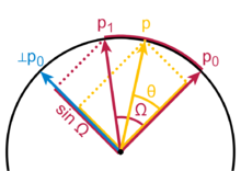
(2 points) show that point $p$ in the Figure above is given by Equation ($*$). You can assume that $\Omega \leq \pi/2$.
Hints: first observe that \begin{equation} p = p_0 \cos{\theta} + {}^{\perp}p_0 \sin\theta \quad (**) \end{equation} You can then write ${}^{\perp}p_0$ in terms of $p_0$, $p_1$ and $\Omega$, and plug this back into $(**)$.
3.2 Equivalence between the Slerp formulae in 3.1 and 2.3 for unit quaternions
Let $q_0$ and $q_1$ be unit quaternions. We start with the Slerp formula in Section 3.1: \begin{aligned} \text{Slerp}(q_0, q_1, t) =&\frac{\sin\left((1-t) \Omega\right)}{\sin \Omega}q_0 + \frac{\sin \left(t \Omega \right)}{\sin \Omega} q_1 \\ =&q_0 \left( \frac{\sin\left((1-t) \Omega\right)}{\sin \Omega} I_q + \frac{\sin \left(t \Omega \right)}{\sin \Omega} q_0^* q_1 \right) \end{aligned} where $I_q = (1, 0, 0, 0)$ is the quaternion which represents the identity rotation; $\Omega = \text{arccos}\left( q_0 \cdot q_1\right)$ (operator $\cdot$ is the inner product in $\mathbb{R}^4$). Note that the above expression has the same form as the Slerp from Section 2.3.
(2 points) show that \begin{equation} \frac{\sin\left((1-t) \Omega\right)}{\sin \Omega} I_q + \frac{\sin \left(t \Omega \right)}{\sin \Omega} q_0^* q_1 = \left( q_0^* q_1 \right)^t \end{equation} which completes the proof of equivalence. You can assume that $\Omega \leq \pi/2$.
Hint: let \begin{equation} q = q_0^* q_1 = \left(\cos{\frac{\alpha}{2}}, \sin{\frac{\alpha}{2}} \pmb{n}\right) \end{equation} and show that $\Omega = \alpha/2$.
4. Controlling rotations using axis-angle
4.1 Convergence of stable first order systems
This is a quick recap of basic control theory. Let $x\in\mathbb{R}$ and $u\in\mathbb{R}$ be the state and input of a first order system. Assuming the system's velocity can be controlled, i.e. $\dot{x} = u$ and the goal is to stabilize $x$ to $x_{\text{ref}}$, then the goal can be achieved by the following control law \begin{equation} u = K(x_{\text{ref}} - x) \end{equation} where $(x_{\text{ref}} - x)$ is called the tracking error and $K \in \mathbb{R}$ the feedback gain.
The control law leads to the following system dynamics \begin{equation} \dot{x} + Kx = K x_{\text{ref}} \end{equation} The convergence of $x$ to $x_{\text{ref}}$ can be shown by inspection.
4.2 Controlling orientation by angular velocity feedback
Let's say frame $A$ is currently at $q_A^W$. You have control of frame $A$'s angular velocity and would like to stabilize it to a reference frame $A_r$ whose orientation is given by $q_{A_r}^W$.
To compute the tracking error, we first compute the relative transform between $A$ and $A_r$ as \begin{equation} q^A_{A_r} = \left(q_A^W\right)^* q_{A_r}^W = \left(\cos{\frac{\theta}{2}}, \sin{\frac{\theta}{2}} \pmb{n}\right) \end{equation}
The control input can then be computed as \begin{equation} u = [^W\omega^{A}]_A = K_{\omega}\left(\theta \pmb{n}\right) \end{equation} where $K_{\omega}$ is a $3 \times 3$ diagonal feedback gain matrix; $[^W\omega^{A}]_A$ is the angular velocity of frame $A$, relative to frame $W$, expressed in frame $A$.
Recall that the angular velocity is also the instantaneous axis of rotation. Therefore, the effect of the above feedback law is to rotate $A$ towards $A_r$ about axis $\pmb{n}$, and the magnitude of this rotation is proportional to the angular tracking error $\theta$. It is important that the error $q^A_{A_r}$ is canonical. Otherwise, the resulting angular velocity could be de-stabilizing if $q^A_{A_r}$ takes the longer path!
Your task is to implement the above feedback controller in CalcAngularVelocity in file rotation.py.
from rotation import RunSimulation

# Reference orientation of frame A, currently set to identity.
R_WA_ref = RotationMatrix()
# Initial orientation of frame A.
R_WA_start = RollPitchYaw(np.pi/4, np.pi/4, np.pi/4).ToRotationMatrix()
# feedback gain, try different values to see its effect on convergence.
kW = 5 * np.eye(3)

t, angular_error, R_WA_log = RunSimulation(R_WA_ref, R_WA_start, kW)
# log playback in meshcat.
vis.delete()
prefix = "control"

# Draw target
AddTriad(vis, "target", prefix, opacity=0.3)

# Draw object
name = "A"
AddTriad(vis, name, prefix, radius=0.015)

# Update object
for R_WA in R_WA_log:
    vis[prefix][name].set_transform(RigidTransform(R_WA, np.zeros(3)).matrix())
    time.sleep(0.002)
# plot angular tracking error, which should converge to 0 exponentially.
plt.figure(dpi=100)
plt.plot(t, angular_error)
plt.grid(True)
plt.xlabel("t [s]")
plt.ylabel("angular tracking error [rad]")
plt.show()
Run tests
import subprocess
# Run the tests
subprocess.run("python3 ./test_pset_5a.py test_results.json", shell=True)

# Print the results json for review
import test_pset_5a
print(test_pset_5a.pretty_format_json_results("test_results.json"))