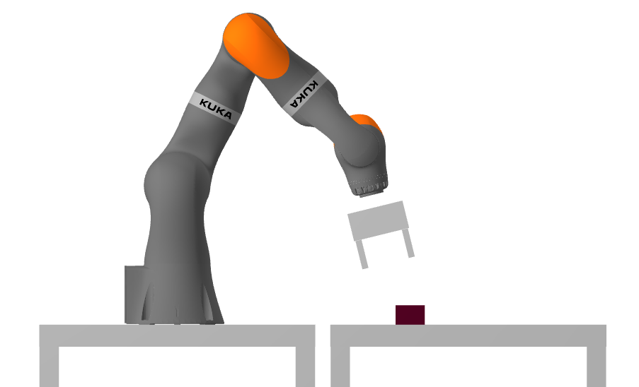
The stage is set. You have your robot. I have a little red foam brick. I'm going to put it on the table in front of your robot, and your goal is to move it to a desired position/orientation on the table. I want to defer the perception problem for one more chapter, and will let you assume that you have access to a perfect measurement of the current position/orientation of the brick. Even without perception, completing this task requires us to build up a basic toolkit for geometry and kinematics; it's a natural place to start.

First, we will establish some terminology and notation for kinematics. This is one area where careful notation can yield dividends, and sloppy notation will inevitably lead to confusion and bugs. The Drake developers have gone to great length to establish and document a consistent multibody notation, which we call "Monogram Notation". The documentation even includes some of the motivation/philosophy behind that notation. I'll use the monogram notation throughout this text.

If you'd like a more extensive background on kinematics than what I provide here, my favorite reference is still Craig05. For free online resources, Chapters 2 and 3 of the 1994 book by Murray et al. (now free online)Murray94 are also excellent, as are the first seven chapters of Modern Robotics by Lynch and ParkLynch17 (they also have excellent accompanying videos). Unfortunately, with three different references you'll get three (slightly) different notations; ours is most similar to Craig05. The monogram notation is developed in some detail in Mitiguy17.

Please don't get overwhelmed by how much background material there is to know! I am personally of the opinion that a clear understanding of just a few basic ideas should make you very effective here. The details will come later, if you need them.

Monogram Notation

The following concepts are disarmingly subtle. I've seen incredibly smart people assume they knew them and then perpetually stumble over notation. I did it for years myself. Take a minute to read this carefully!

Perhaps the most fundamental concept in geometry is the concept of a point. Points occupy a position in space, and they can have names, e.g. point $A$, $C$, or more descriptive names like $B_{cm}$ for the center of mass of body $B$. We'll denote the position of the point by using a position vector $p^A$; that's $p$ for position, and not for point, because other geometric quantities can also have a position.

But let's be more careful. Position is actually a relative quantity. Really, we should only ever write the position of two points relative to each other. We'll use e.g. $^Ap^C$ to denote the position of $C$ measured from $A$. The left superscript looks mighty strange, but we'll see that it pays off once we start transforming points.

Every time we describe the (relative) position as a vector of numbers, we need to be explicit about the frame we are using, specifically the "expressed-in" frame. All of our frames are defined by orthogonal unit vectors that follow the "right-hand rule". We'll give a frame a name, too, like $F$. If I want to write the position of point $C$ measured from point $A$, expressed in frame $F$, I will write $^Ap^C_F$. If I ever want to get just a single component of that vector, e.g. the $x$ component, then I'll use $^Ap^C_{F_x}$. In some sense, the "expressed-in" frame is an implementation detail; it is only required once we want to represent the multibody quantity as a vector (e.g. in the computer).

That is seriously heavy notation. I don't love it myself, but it's the most durable I've got, and we'll have shorthand for when the context is clear.

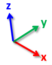There are a few very special frames. We use $W$ to denote the world frame. We think about the world frame in Drake using vehicle coordinates (positive $x$ to the front, positive $y$ to the left, and positive $z$ is up). The other particularly special frames are the body frames: every body in the multibody physics engine has a unique frame attached to it. We'll typically use $B_i$ to denote the frame for body $i$.

Frames have a position, too -- it coincides with the frame origin. So it is perfectly valid to write $^Wp^A_W$ to denote the position of point $A$ measured from the origin of the world frame, expressed in the world frame. Here is where the shorthand comes in. If the position of a quantity is measured from a frame, and expressed in the same frame, then we can safely omit the subscript. $^Fp^A \equiv {^Fp^A_F}$. Furthermore, if the "measured from" field is omitted, then we assume that the point is measured from $W$, so $p^A \equiv {}^Wp^A_W$.

Frames also have an orientation. We'll use $R$ to denote a rotation, and follow the same notation, writing $^BR^A$ to denote the orientation of frame $A$ measured from frame $B$. Unlike vectors, pure rotations do not have an additional "expressed in" frame.

A frame $F$ can be specified completely by a position and rotation measured from another frame. Taken together, we call the position and orientation a spatial pose, or just pose. A spatial transform, or just transform, is the "verb form" of pose. In Drake we use RigidTransform to represent a pose/transform, and denote it with the letter $X$. $^BX^A$ is the pose of frame $A$ measured from frame $B$. When we talk about the pose of an object $O$, without mentioning a reference frame explicitly, we mean $^WX^O$ where $O$ is the body frame of the object. We do not use the "expressed in" frame subscript for pose; we always want the pose expressed in the reference frame.

The Drake documentation also discusses how to use this notation in code. In short, $^Bp^A_C$ is written p_BA_C, ${}^BR^A$ as R_BA, and ${}^BX^A$ as X_BA. It works, I promise.

Spatial Algebra

Here is where we start to see the pay-off from our heavy notation, as we define the rules of converting positions, rotations, poses, etc. between different frames. Without the notation, this invariably involves me with my right hand in the air making the "right-hand rule", and my head twisting around in space. With the notation, it's a simple matter of lining up the symbols properly, and we're more likely to get the right answer!

Here are the basic rules of algebra for our spatial quantities:

Positions expressed in the same frame can be added when their reference and target symbols match: \begin{equation}{}^Ap^B_F + {}^Bp^C_F = {}^Ap^C_F.\end{equation} Addition is commutative, and the additive inverse is well defined: \begin{equation}{}^Ap^B_F = - {}^Bp^A_F.\end{equation} Those should be pretty intuitive; make sure you confirm them for yourself.
Multiplication by a rotation can be used to change the "expressed in" frame: \begin{equation}{}^Ap^B_G = {}^GR^F {}^Ap^B_F.\end{equation} You might be surprised that a rotation alone is enough to change the expressed-in frame, but it's true. The position of the expressed-in frame does not affect the relative position between two points.
Rotations can be multiplied when their reference and target symbols match: \begin{equation}{}^AR^B \: {}^BR^C = {}^AR^C.\end{equation} The inverse operation is also simply defined: \begin{equation}\left[{}^AR^B\right]^{-1} = {}^BR^A.\end{equation} When the rotation is represented as a rotation matrix, this is literally the matrix inverse, and since rotation matrices are orthonormal, we also have $R^{-1}=R^T.$
Transforms bundle this up into a single, convenient notation when positions are measured from a frame (and the same frame they are expressed in): \begin{equation}{}^Gp^A = {}^GX^F {}^Fp^A = {}^Gp^F + {}^Fp^A_G = {}^Gp^F + {}^GR^F {}^Fp^A.\end{equation}
Transforms compose: \begin{equation}{}^AX^B {}^BX^C = {}^AX^C,\end{equation} and have an inverse \begin{equation}\left[{}^AX^B\right]^{-1} = {}^BX^A.\end{equation} Please note that for transforms, we generally do not have that $X^{-1}$ is $X^T,$ though it still has a simple form.

In practice, transforms are implemented using homogenous coordinates, but for now I'm happy to leave that as an implementation detail.

From camera frame to world frame

Add a figure here.

Imagine that I have a depth camera mounted in a fixed pose in my workspace. Let's call the camera frame $C$ and denote its pose in the world with ${}^WX^C$.

A depth camera returns points in the camera frame. Therefore, we'll write this position of point $P_i$ with ${}^Cp^{P_i}$. If we want to convert the point into the world frame, we simply have $$p^{P_i} = X^C {}^Cp^{P_i}.$$

This is a work-horse operation for us. We often aim to merge points from multiple cameras (typically in the world frame), and always need to somehow relate the frames of the camera with the frames of the robot. The inverse transform, ${}^CX^W$, which projects world coordinates into the camera frame, is often called the camera "extrinsics".

Representations for 3D rotation

In the spatial algebra above, I've written the rules for rotations using an abstract notion of rotation. But in order to implement this algebra in code, we need to decide how we are going to represent those representations with a small number of real values. There are many possible representations of 3D rotations, they are each good for different operations, and unfortunately, there is no one representation to rule them all. (This is one of the many reasons why everything is better in 2D!) Common representations include

3$\times$3 rotation matrices,
Euler angles (e.g. roll-pitch-yaw),
axis angle (aka "exponential coordinates"), and
unit quaternions.

In Drake, we provide all of these representations, and make it easy to convert back and forth between them.

A 3$\times$3 rotation matrix is an orthonormal matrix with columns formed by the $x-$, $y-$, and $z-$axes. Specifically, the first column of the transform ${}^GR^F$ has the $x-$axis of frame $F$ expressed in $G$ in the first column, etc.

Euler angles specify a 3D rotation by a series of rotations around the $x$, $y$, and $z$ axes. The order of these rotations matters; and many combinations can be used to describe any 3D rotation. This is why we use RollPitchYaw in the code (preferring it over the more general term "Euler angle") and document it carefully. Roll is a rotation around the $x$-axis, pitch is a rotation around the $y$-axis, and yaw is a rotation around the $z$-axis; this is also known as "extrinsic X-Y-Z" Euler angles.

Axis angles describe a 3D rotation by a scalar rotation around an arbitrary vector axis using three numbers: the direction of the vector is the axis, and the magnitude of the vector is the angle. You can think of unit quaternions as a form of axis angles that have been carefully normalized to be unit length and have magical properties. My favorite careful description of quaternions is probably chapter 1 of Stillwell08.

Why all of the representations? Shouldn't "roll-pitch-yaw" be enough? Unfortunately, no. The limitation is perhaps most easily seen by looking at the coordinate changes from roll-pitch-yaw to/from a rotation matrix. Any roll-pitch-yaw can be converted to a rotation matrix, but the inverse map has a singularity. In particular, when the pitch angle is $\frac{\pi}{2}$, then roll and yaw are now indistinguishable. This is described very nicely, along with its physical manifestation in "gimbal lock" in this video. Similarly, the direction of the vector in the axis-angle representation in not uniquely defined when the rotation angle is zero. These singularities become problematic when we start taking derivatives of rotations, for instance when we write the equations of motion. It is now well understood Stillwell08 that it requires at least four numbers to properly represent the group of 3D rotations; the unit quaternion is the most common four-element representation.

Forward kinematics

The spatial algebra gets us pretty close to what we need for our pick and place algorithm. But remember that the interface we have with the robot reports measured joint positions, and expects commands in the form of joint positions. So our remaining task is to convert between joint angles and cartesian frames. We'll do this in steps, the first step is to go from joint positions to cartesian frames: this is known as forward kinematics.

Throughout this text, we will refer to the joint positions of the robot (also known as "configuration" of the robot) using a vector $q$. If the configuration of the scene includes objects in the environment as well as the robot, we would use $q$ for the entire configuration vector, and use e.g. $q_{robot}$ for the subset of the vector corresponding to the robot's joint positions. Therefore, the goal of forward kinematics is to produce a map: \begin{equation}X^G = f_{kin}^G(q).\end{equation} Moreover, we'd like to have forward kinematics available for any frame we have defined in the scene. Our spatial notation and spatial algebra makes this computation relatively straight-forward.

The kinematic tree

In order to facilitate kinematics and related multibody computations, the MultibodyPlant organizes all of the bodies in the world into a tree topology. Every body (except the world body) has a parent, which it is connected to via either a Joint or a "floating base".

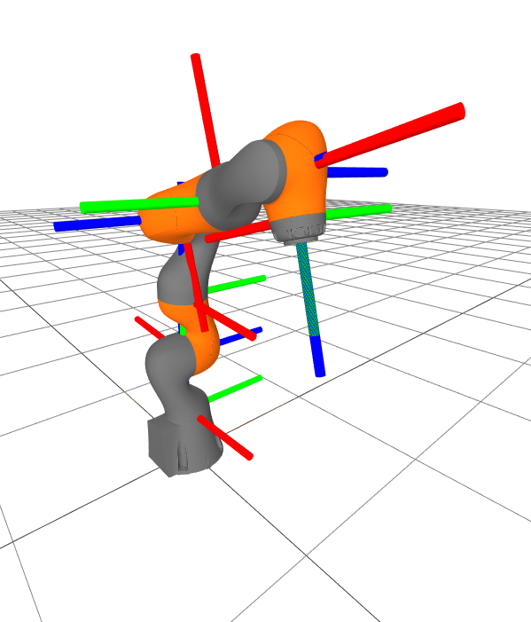
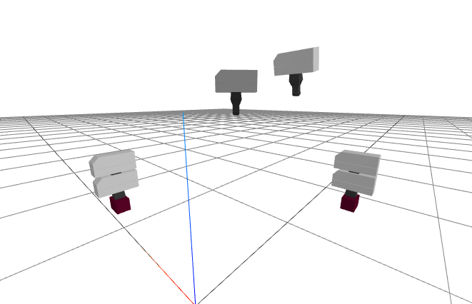
Inspecting the kinematic tree

Drake provides some visualization support for inspecting the kinematic tree data structure. The kinematic tree for an iiwa is more of a vine than a tree (it's a serial manipulator), but the tree for the dexterous hands are more interesting. I've added our brick to the example, too, so that you can see that a "free" body is just another branch off the world root node.

Insert topology visualization here (once it is better)

Every Joint and "floating base" has some number of position variables associated with it -- a subset of the configuration vector $q$ -- and knows how to compute the configuration dependent transform across the joint from the child joint frame $J_C$ to the parent joint frame $J_P$: ${}^{J_P}X^{J_C}(q)$. Additionally, the kinematic tree defines the (fixed) transforms from the joint frame to the child body frame, ${}^CX^{J_C}$, and from the joint frame to the parent frame, ${}^PX^{J_P}$. Altogether, we can compute the configuration transform between any one body and its parent, $${}^PX^C(q) = {}^PX^{J_P} {}^{J_P}X^{J_C}(q) {}^{J_C}X^C.$$

Examples or links to specifying the kinematic tree in URDF, SDF, etc...

You might be tempted to think that every time you add a joint to the MultibodyPlant, you are adding a degree of freedom. But it actually works the other way around. Every time you add a body to the plant, you are adding many degrees of freedom. But you can then add joints to remove those degrees of freedom; joints are constraints. "Welding" the robot's base to the world frame removes all of the floating degrees of freedom of the base. Adding a rotational joint between a child body and a parent body removes all but one degree of freedom, etc.

Forward kinematics for pick and place

In order to compute the pose of the gripper in the world, $X^G$, we simply query the parent of the gripper frame in the kinematic tree, and recursively compose the transforms until we get to the world frame.

Kinematic frames on the iiwa (left) and the WSG (right). For each frame, the positive $x$ axis is in red, the positive $y$ axis is in green, and the positive $z$ axis is in blue. It's (hopefully) easy to remember: XYZ $\Leftrightarrow$ RGB.

Forward kinematics for the gripper frame

Let's evaluate the pose of the gripper in the world frame: $X^G$. We know that it will be a function of configuration of the robot, which is just a part of the total state of the MultibodyPlant (and so is stored in the Context). The following example shows you how it works.

The key lines are

gripper = plant.GetBodyByName("body", wsg)
pose = plant.EvalBodyPoseInWorld(context, gripper)

Behind the scenes, the MultibodyPlant is doing all of the spatial algebra we described above to return the pose (and also some clever caching because you can reuse much of the computation when you want to evaluate the pose of another frame on the same robot).

Forward kinematics of "floating-base" objects

Consider the special case of having a MultibodyPlant with exactly one body added, and no joints. The kinematic tree is simply the world frame, the body frame, and they are connected by the "floating base". What does the forward kinematics function: $$X^B = f_{kin}^B(q),$$ look like in that case? If $q$ is already representing the floating-base configuration, is $f^B_{kin}$ just the identity function?

This gets into the subtle points of how we represent transforms, and how we represent 3D rotations in particular. Although we use rotation matrices in our RigidTransform class, in order to make the spatial algebra efficient, we actually use unit quaternions in the configuration vector $q,$ and in the Context in order to have a compact representation.

As a result, for this example, the software implementation of the function $f_{kin}^B$ is precisely the function that converts the position $\times$ unit quaternion representation into the pose (position $\times$ rotation matrix) representation.

Differential kinematics (Jacobians)

The forward kinematics machinery gives us the ability to compute the pose of the gripper and the pose of the object, both in the world frame. But if our goal is to move the gripper to the object, then we should understand how changes in the joint angles relate to changes in the gripper pose. This is traditionally referred to as "differential kinematics".

At first blush, this is straightforward. The change in pose is related to a change in joint positions by the (partial) derivative of the forward kinematics: \begin{equation}dX^B = \pd{f_{kin}^B(q)}{q} dq = J^B(q)dq. \label{eq:jacobian}\end{equation} Partial derivatives of a function are referred to as "Jacobians" in many fields; in robotics it's rare to refer to derivatives of the kinematics as anything else.

All of the subtlety, again, comes in because of the multiple representations that we have for 3D rotations (rotation matrix, unit quaternions, ...). While there is no one best representation for 3D rotations, it is possible to have one canonical representation for differential rotations. Without any concern for singularities nor loss of generality, we can represent the rate of change in pose using a six-component vector for spatial velocity: \begin{equation}{}^AV^B_C = \begin{bmatrix} {}^A\omega^B_C \\ {}^A\text{v}^B_C \end{bmatrix}.\end{equation} ${}^AV^B_C$ is the spatial velocity (also known as a "twist") of frame $B$ measured in frame $A$ expressed in frame $C$, ${}^A\omega^B_C \in \Re^3$ is the angular velocity (of frame $B$ measured in $A$ expressed in frame $C$), and ${}^A\text{v}^B_C \in \Re^3$ is the translational velocity (along with the same shorthands as for positions). The angular velocity is a 3D vector (with $w_x$, $w_y$, $w_z$ components); the magnitude of this vector represents the angular speed and the direction represents the (instantaneous) axis of rotation. It's tempting to think of it as the time derivatives of roll, pitch, and yaw, but that's not true; it can easily be converted into that representation through a nonlinear change of coordinates. Spatial velocities fit nicely into our spatial algebra:

Angular velocities add (when the frames match): \begin{equation} {}^A\omega^B_F + {}^B\omega^C_F = {}^A\omega^C_F,\end{equation} (this deserves to be verified) and have the additive inverse, ${}^A\omega^C_F = - {}^C\omega^A_F,$.
Rotations can be used to change between the "expressed-in" frames: \begin{equation} {}^A\text{v}^B_G = {}^GR^F {}^A\text{v}^B_F, \qquad {}^A\omega^B_G = {}^GR^F {}^A\omega^B_F.\end{equation}
Translational velocities compose across frames with: \begin{equation}{}^A\text{v}^C_F = {}^A\text{v}^B_F + {}^B\text{v}^C_F + {}^A\omega^B_F \times {}^Bp^C_F.\end{equation}
This can be derived in a few steps (click the triangle to expand)
Differentiating $${}^Ap^C = {}^AX^B {}^Bp^C = {}^Ap^B + {}^AR^B {}^Bp^C,$$ yields \begin{align} {}^A\text{v}^C =& {}^A\text{v}^B + {}^A\dot{R}^B {}^Bp^C + {}^AR^B {}^B\text{v}^C \nonumber \\ =& {}^A\text{v}^B_A + {}^A\dot{R}^B {}^BR^A {}^Bp^C_A + {}^B\text{v}^C_A.\end{align} Allow me to write $\dot{R}R^{-1}$ for ${}^A\dot{R}^B {}^BR^A$ (dropping the frames for a moment). It turns out that $\dot{R}R^{-1}$, is always a skew-symmetric matrix. To see this, differentiate $RR^T = I$ to get $$\dot{R}R^T + R\dot{R}^T = 0 \Rightarrow \dot{R}R^T = - R\dot{R}^T \Rightarrow \dot{R} R^T = - (\dot{R} R^T)^T,$$ which is the definition of a skew-symmetric matrix. Any 3$\times$3 skew-symmetric matrix can be parameterized by three numbers (we'll use the three-element vector $\omega$), and can be written as a cross product, so $\dot{R}R^Tp = \omega \times p.$

Multiply the right and left sides by ${}^FR^A$ to change the expressed-in frame, and we have our result.
This reveals that additive inverse for translational velocities is not obtained by switching the reference and measured-in frames; it is slightly more complicated: \begin{equation}-{}^A\text{v}^B_F = {}^B\text{v}^A_F + {}^A\omega^B_F \times {}^Bp^A_F.\end{equation} .

If you're familiar with "screw theory" (as used in, e.g. Murray94 and Lynch17), click the triangle to see how those conventions are related.

Screw theory (as used in, e.g. Murray94 and Lynch17) often uses a particular form of our spatial velocity referred to as "spatial velocity in the space frame" / "spatial twists" that can be useful in a number of computations. This quantity is ${}^AV^{B_A}$, where $B_A$ is the frame rigidly attached on body $B$ (so ${}^BV^{B_A} = 0$) that is instantaneously in the same pose as $A$ (so ${}^Ap^{B_A} = 0$, ${}^AR^{B_A} = I$) Lynch17. These conditions reduce to \begin{equation}{}^AV^{B_A} = \begin{bmatrix} {}^A\omega^{B_A} \\ {}^A\text{v}^{B_A} \end{bmatrix} = \begin{bmatrix} {}^A\omega^{B_A} + {}^{B_A}\omega^B_{A} \\ {}^A\text{v}^B + {}^B\text{v}^{B_A}_A + {}^A\omega^B \times {}^Bp^{B_A}_A \end{bmatrix} = \begin{bmatrix} {}^A \omega^{B} \\ {}^A\text{v}^B - {}^A\omega^B \times {}^Ap^{B} \end{bmatrix}.\end{equation}

Why is it that we can get away with just three components for angular velocity, but not for rotations? Using the magnitude of an axis-angle representation to denote an angle is degenerate because our representation of angles should be periodic in $2\pi$, but using the magnitude of the angular velocity is ok because angular velocities take values from $(-\infty, \infty)$ without wrapping.

There is one more velocity to be aware of: I'll use $v$ to denote the generalized velocity vector of the plant, which is closely related to the time-derivative of $q$ (see below). While a spatial velocity $^AV^B$ is six components, a translational or angular velocity, $^B\text{v}^C$ or $^B\omega^C$, is three components, the generalized velocity vector is whatever size it needs to be to encode the time derivatives of the configuration variables, $q$. For the iiwa welded to the world frame, that means it has seven components. I've tried to be careful to typeset each of these v's differently throughout the notes. Almost always the distinction is also clear from the context.

Don't assume $\dot{q} \equiv v$

The unit quaternion representation is four components, but these must form a "unit vector" of length 1. Rotation matrices are 9 components, but they must form an orthonormal matrix with $\det(R)=1$. It's pretty great that for the time derivative of rotation, we can use an unconstrained three component vector, what we've called the angular velocity vector, $\omega$. And you really should use it; getting rid of that constraint makes both the math and the numerics better.

But there is one minor nuisance that this causes. We tend to want to think of the generalized velocity as the time derivative of the generalized positions. This works when we have only our iiwa in the model, and it is welded to the world frame, because all of the joints are revolute joints with a single degree of freedom each. But we cannot assume this in general; when floating-base rotations part of the generalized position. As evidence, here is a simple example that loads exactly one rigid body into the MultibodyPlant, and then prints its Context.

The output looks like this:

Context
--------
Time: 0
States:
  13 continuous states
    1 0 0 0 0 0 0 0 0 0 0 0 0

plant.num_positions() = 7
plant.num_velocities() = 6


Position names: ['$world_base_link_qw', '$world_base_link_qx', '$world_base_link_qy', '$world_base_link_qz', '$world_base_link_x', '$world_base_link_y', '$world_base_link_z']
Velocity names: ['$world_base_link_wx', '$world_base_link_wy', '$world_base_link_wz', '$world_base_link_vx', '$world_base_link_vy', '$world_base_link_vz']

You can see that this system has 13 total state variables. 7 of them are positions, $q$, because we use unit quaternions in the position vector. But we have just 6 velocities, $v$; we use angular velocities in the velocity vector. Clearly, if the length of the vectors don't even match, we do not have $\dot{q} = v$.

It is not difficult to deal with this representational detail; Drake provides the MultibodyPlant methods MapQDotToVelocity and MapVelocityToQDot to go back and forth between them. But you have to remember to use them!

Due to the multiple possible representations of 3D rotation, and the potential difference between $\dot{q}$ and $v$, there are actually many different kinematic Jacobians possible. You may hear the terms "analytic Jacobian", which refers to the explicit partial derivative of the forward kinematics (as written in \eqref{eq:jacobian}), and "geometric Jacobian" which replaces 3D rotations on the left-hand side with spatial velocities. In Drake's MultibodyPlant, we currently offer the geometric Jacobian versions via

CalcJacobianAngularVelocity,
CalcJacobianTranslationalVelocity, and
CalcJacobianSpatialVelocity,

with each taking an argument to specify whether you'd like the Jacobian with respect to $\dot{q}$ or $v$. If you really like the analytical Jacobian, you could get it (much less efficiently) using Drake's support for automatic differentiation.

Kinematic Jacobians for pick and place

Let's repeat the setup from above, but we'll print out the Jacobian of the gripper frame, measured from the world frame, expressed in the world frame.

Differential inverse kinematics

The geometric Jacobian provides a linear relationship between generalized velocity and spatial velocity: \begin{equation}V^G = J^G(q)v.\end{equation} Can this gives us what we need to produce changes in gripper frame $G$? If I have a desired gripper frame velocity $V^{G_d}$, then how about commanding a joint velocity $v = \left[J^G(q)\right]^{-1} V^{G_d}$?

The Jacobian pseudo-inverse

Any time you write a matrix inverse, it's important to check that the matrix is actually invertible. As a first sanity check: what are the dimensions of $J^G(q)$? We know the spatial velocity has six components. Our gripper frame is welded directly on the last link of the iiwa, and the iiwa has seven positions, so we have $J^G(q_{iiwa}) \in \Re^{6 \times 7}.$ The matrix is not square, so does not have an inverse. But having more degrees of freedom than the desired spatial velocity requires (more columns than rows) is actually the good case, in the sense that we might have many solutions for $v$ that can achieve a desired spatial velocity. To choose one of them (the minimum-norm solution), we can consider using the Moore-Penrose pseudo-inverse, $J^+$, instead: \begin{equation}v = [J^G(q)]^+V^{G_d}.\end{equation}

The pseudo-inverse is a beautiful mathematical concept. When the $J$ is square and full-rank, the pseudo-inverse returns the true inverse of the system. When there are many solutions (here many joint velocities that accomplish the same end-effector spatial velocity), then it returns the minimum-norm solution (the joint velocities that produce the desired spatial velocity which are closest to zero in the least-squares sense). When there is no exact solution, it returns the joint velocities that produce an spatial velocity which is as close to the desired end-effector velocity as possible, again in the least-squares sense. So good!

Our first end-effector "controller"

Let's write a simple controller using the pseudo-inverse of the Jacobian. First, we'll write a new LeafSystem that defines one input port (for the iiwa measured position), and one output port (for the iiwa joint velocity command). Inside that system, we'll ask MultibodyPlant for the gripper Jacobian, and compute the joint velocities that will implement a desired gripper spatial velocity.

To keep things simple for this first example, we'll just command a constant gripper spatial velocity, and only run the simulation for a few seconds.

Note that we do have to add one additional system into the diagram. The output of our controller is a desired joint velocity, but the input that the iiwa controller is expecting is a desired joint position. So we will insert an integrator in between.

I don't expect you to understand every line in this example, but it's worth finding the important lines and making sure you can change them and see what happens!

Congratulations! Things are really moving now.

Invertibility of the Jacobian

There is a simple check to understand when the pseudo-inverse can give an exact solution for any spatial velocity (achieving exactly the desired spatial velocity): the rank of the Jacobian must be equal to the number of rows (sometimes called "full row rank"). In this case, we need $\rank(J) = 6$. But assigning an integer rank to a matrix doesn't tell the entire story; for a real robot with (noisy) floating-point joint positions, as the matrix gets close to losing rank, the (pseudo-)inverse starts to "blow-up". A better metric, then, is to watch the smallest singular value; as this approaches zero, the norm of the pseudo-inverse will approach infinity.

Invertibility of the gripper Jacobian

You might have noticed that I printed out the smallest singular value of $J^G$ in one of the previous examples. Take it for another spin. See if you can find configurations where the smallest singular value gets close to zero.

Here's a hint: try some configurations where the arm is very straight, (e.g. driving joint 2 and 4 close to zero).

Another good way to find the singularities are to use your pseudo-inverse controller to send gripper spatial velocity commands that drive the gripper to the limits of the robot's workspace. Try it and see! In fact, this can happen easily in practice when using end-effector commands, and we will work hard to avoid it.

Configurations $q$ for which $\rank(J(q_{iiwa})) < 6$ for a frame of interest (like our gripper frame $G$) are called kinematic singularities. Try to avoid going near them if you are using end-effector control! The iiwa has many virtues, but admittedly its kinematic workspace is not one of them. Trust me, if you try to get a big Kuka to reach into a little kitchen sink all day, every day, then you will spend a non-trivial amount of time thinking about avoiding singularities.

In practice, things can get a lot better if we stop bolting our robot base to a fixed location in the world. Mobile bases add complexity, but they are wonderful for improving the kinematic workspace of a robot.

Are kinematic singularities real?

A natural question when discussing singularities is whether they are somehow real, or whether they are somehow an artifact of the analysis. Does the robot blow up? Does it get mechanically stuck? Or is it just our math that is broken? Perhaps it is useful to look at an extremely simple case.

Imagine a two-link arm, where each link has length one. Then the kinematics reduce to $$p^G = \begin{bmatrix} c_0 + c_{0+1} \\ s_0 + s_{0 + 1} \end{bmatrix},$$ where I've used the (very common) shorthard $s_0$ for $\sin(q_0)$, $c_0$ for $\cos(q_0)$, $s_{0+1}$ for $\sin(q_0+q_1),$ etc. The translational Jacobian is $$J^G(q) = \begin{bmatrix} -s_0 - s_{0+1} & -s_{0 + 1} \\ c_0 + c_{0 + 1} & c_{0 + 1} \end{bmatrix},$$ and as expected, it loses rank when the arm is at full extension (e.g. when $q_0 = q_1 = 0$ which implies the first row is zero).

Click here for the animation.

Let's move the robot along the $x$-axis, by taking $q_0(t) = 1-t,$ and $q_1(t) = -2 + 2t$. This clearly visits the singularity $q_0 = q_1 = 0$ at time 1, and then leaves again without trouble. In fact, it does all this with a constant joint velocity ($\dot{q}_0=-1, \dot{q}_1=2$)! The resulting trajectory is $$p^G(t) = \begin{bmatrix} 2\cos(1-t) \\ 0 \end{bmatrix}.$$

There are a few things to understand. At the singularity, there is nothing that the robot can do to move its gripper farther in positive $x$ -- that singularity is real. But it is also true that there is no way for the robot to move instantaneously back in the direction of $-x.$ The Jacobian analysis is not an approximation, it is a perfect description of the relationship between joint velocities and gripper velocities. However, just because you cannot achieve an instantaneous velocity in the backwards direction, it does not mean you cannot get there! At $t=1$, even though the joint velocities are constant, and the translational Jacobian is singular, the robot is accelerating in $-x$, $\ddot{p}^G_{W_x}(t) = -2\cos(1-t).$

Update this to use the two-link iiwa (like i've done in the qp_diff_ik notebook). The link lengths aren't *quite* one to one, but it's close. could have a point on the second link that is the right distance away, or just add the ratio logic here.

For the cases when the Jacobian does not have a unique inverse, there is an interesting subtlety to be aware of regarding integrability. Let's start our robot in at time zero in a joint configuration, $q(0)$ with a corresponding in an end-effector pose $X^G(0)$. Now let us execute an end-effector trajectory using the pseudo-inverse controller that moves along a closed-path in the task space, coming back to the original end-effector pose at time one: $X^G(1) = X^G(0)$. Unfortunately, there is no guarantee that $q(1) = q(0)$; this is not simply due to numerical errors in our numerical implementation, it is well known that the pseudo-inverse does not in general produce an integrable function. Mussa-Ivaldi91 discusses this thoroughly, and proposed a weighted pseudo-inverse that can restore the integrability conditions by means of a virtual "compliance function".

Defining the grasp and pre-grasp poses

I'm going to put my red foam brick on the table. Its geometry is defined as a 7.5cm x 5cm x 5cm box. For reference, the distance between the fingers on our gripper in the default "open" position is 10.7cm. The "palm" of the gripper is 3.625cm from the body origin, and the fingers are 8.2cm long.

To make things easy to start, I'll promise to set the object down on the table with the object frame's $z$-axis pointing up (aligned with the world $z$ axis), and you can assume it is resting on the table safely within the workspace of the robot. But I reserve the right to give the object arbitrary initial yaw. Don't worry, you might have noticed that the seventh joint of the iiwa will let you rotate your gripper around quite nicely (well beyond what my human wrist can do).

Observe that visually the box has rotational symmetry -- I could always rotate the box 90 degrees around its $x$-axis and you wouldn't be able to tell the difference. We'll think about the consequences of that more in the next chapter when we start using perception. But for now, we are ok using the omniscient "cheat port" from the simulator which gives us the unambiguous pose of the brick.

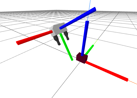
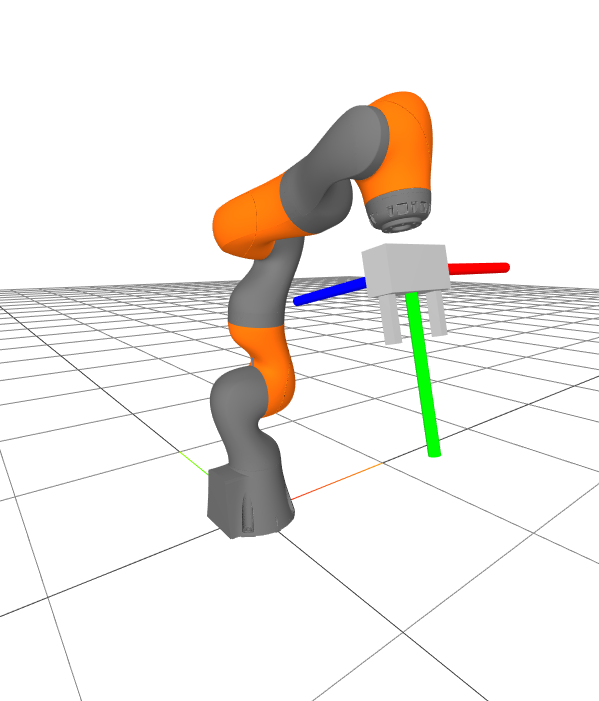
The gripper frame and the object frame. For each frame, the positive $x$ axis is in red, the positive $y$ axis is in green, and the positive $z$ axis is in blue (XYZ $\Leftrightarrow$ RGB).

Take a careful look at the gripper frame in the figure above, using the colors to understand the axes. Here is my thinking: Given the size of the hand and the object, I want the desired position (in meters) of the object in the gripper frame, $${}^{G_{grasp}}p^O = \begin{bmatrix} 0 \\ 0.11 \\ 0 \end{bmatrix}, \qquad {}^{G_{pregrasp}}p^O = \begin{bmatrix} 0 \\ 0.2 \\ 0 \end{bmatrix}.$$ Recall that the logic behind a pregrasp pose is to first move to safely above the object, if our only gripper motion that is very close to the object is a straight translation from the pregrasp pose to the grasp pose and back, then it allows us to mostly avoid having to think about collisions (for now). I want the orientation of my gripper to be set so that the positive $z$ axis of the object aligns with the negative $y$ axis of the gripper frame, and the positive $x$ axis of the object aligns with the positive $z$ axis of the gripper. We can accomplish that with $${}^{G_{grasp}}R^O = \text{MakeXRotation}\left(\frac{\pi}{2}\right) \text{MakeZRotation} \left(\frac{\pi}{2}\right).$$ I admit I had my right hand in the air for that one! Our pregrasp pose will have the same orientation as our grasp pose.

Computing grasp and pregrasp poses

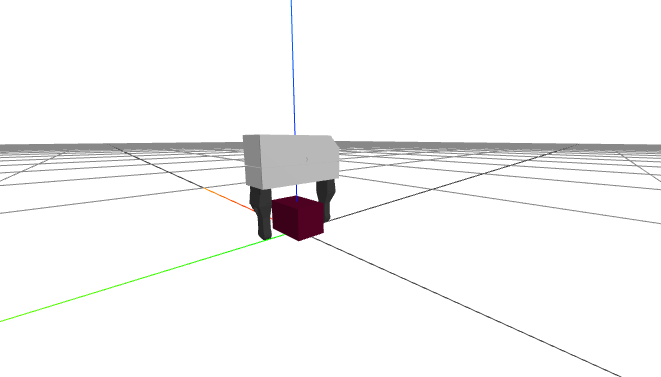
Here is a simple example of loading a floating Schunk gripper and a brick, computing the grasp / pregrasp pose (drawing out each transformation clearly), and rendering the hand relative to the object.

I hope you can see the value of having good notation at work here. My right hand was in the air when I was deciding what a suitable relative pose for the object in the hand should be (when writing the notes). But once that was decided, I went to type it in and everything just worked.

A pick and place trajectory

We're getting close. We know how to produce desired gripper poses, and we know how to change the gripper pose instantaneously using spatial velocity commands. Now we need to specify how we want the gripper poses to change over time, so that we can convert our gripper poses into spatial velocity commands.

Let's define all of the "keyframe" poses that we'd like the gripper to travel through, and time that it should visit each one. The following example does precisely that.

A plan "sketch"

Keyframes of the gripper. The robot's base will be at the origin, so we're looking over the (invisible) robot's shoulder here. The hand starts in the "initial" pose near the center, moves to the "prepick" to "pick" to "prepick" to "clearance" to "preplace" to "place" and finally back to "preplace".

timeline graphic here, from time zero, to pre-grasp, to grasp, to

How did I choose the times? I started everything at time, $t=0$, and listed the rest of our times as absolute (time from zero). That's when the robot wakes up and sees the brick. How long should we take to transition from the starting pose to the pregrasp pose? A really good answer might depend on the exact joint speed limits of the robot, but we're not trying to move fast yet. Instead I chose a conservative time that is proportional to the total Euclidean distance that the hand will travel, say $k=10~s/m$ (aka $10~cm/s$): $$t_{pregrasp} = k \left\|{}^{G_0}p^{G_{pregrasp}}\right\|_2.$$ I just chose a fixed duration of 2 seconds for the transitions from pregrasp to grasp and back, and also left 2 seconds with the gripper stationary for the segments where the fingers needs to open/close.

There are a number of ways one might represent a trajectory computationally. We have a pretty good collection of trajectory classes available in Drake. Many of them are implemented as splines -- piecewise polynomial functions of time. Interpolating between orientations requires some care, but for positions we can do a simple linear interpolation between each of our keyframes. That would be called a "first-order hold", and it's implemented in Drake's PiecewisePolynomial class. For rotations, we'll use something called "spherical linear interpolation" or slerp, which is implemented in Drake's PiecewiseQuaternionSlerp, and which you can explore in this exercise. The PiecewisePose class makes it convenient to construct and work with the position and orientation trajectories together.

Grasping with trajectories

There are a number of ways to visualize the trajectory when it's connected to 3D. I've plotted the position trajectory as a function of time below.

With 3D data, you can plot it in 3D. But my favorite approach is as an animation in our 3D renderer! Make sure you try the "Open controls>Animation" interface. You can pause it and then scrub through the trajectory using the time slider.

For a super interesting discussion on how we might visualize the 4D quaternions as creatures trapped in 3D, you might enjoy this series of "explorable" videos.

One final detail -- we also need a trajectory of gripper commands (to open and close the gripper). We'll use a first-order hold for that, as well.

Differential inverse kinematics with constraints

Our solution above works in many cases. We could potentially move on. But with just a little more work, we can get a much more robust solution... one that we will be happy with for many chapters to come.

So what's wrong with the pseudo-inverse controller? You won't be surprised when I say that it does not perform well around singularities. When the minimum singular value of the Jacobian gets small, that means that some values in the inverse get very large. If you ask our controller to track a seemingly reasonable end-effector spatial velocity, then you might have extremely large velocity commands that result.

There are other important limitations, though, which are perhaps more subtle. The real robot has constraints, very real constraints on the joint angles, velocities, accelerations, and torques. If you, for instance, send a velocity command to the iiwa controller that cannot be followed, that velocity will be clipped. In the mode we are running the iiwa (joint-impedance mode), the iiwa doesn't know anything about your end-effector goals. So it will very likely simply saturate your velocity commands independently joint by joint. The result, I'm afraid, will not be as convenient as a slower end-effector trajectory. Your end-effector could run wildly off course.

Since we know the limits of the iiwa, a better approach is to take these constraints into account at the level of our controller. It's relatively straight-forward to take position, velocity, and acceleration constraints into account; torque constraints require a full dynamics model so we won't worry about them yet here (but they can plug in naturally to this framework).

Pseudo-inverse as an optimization

I introduced the pseudo-inverse as having almost magical properties: it returns an exact solution when one is available, or the best possible solution (in the least-squares norm) when one is not. These properties can all be understood by realizing that the pseudo-inverse is just the optimal solution to a least-squares optimization problem: \begin{equation} \min_v \left|J^G(q)v - V^{G_d}\right|^2_2. \end{equation} When I write an optimization of this form, I will refer to $v$ as the decision variable(s), and I will use $v^*$ to denote the optimal solution (the value of the decision variables that minimizes the cost). This particular optimization problem has a closed-form solution, which just happens to be exactly what is provided by the pseudo-inverse: $$v^* = \left[ J^G(q) \right]^+V^{G_d}.$$ More generally, we will expect to employ numerical methods to solve optimization problems.

Optimization is an incredibly rich topic, and we will put many tools from optimization to use over the course of this text. For a beautiful rigorous but accessible treatment of convex optimization, I highly recommend Boyd04a; it is free online and even reading the first chapter can be incredibly valuable. For a very short introduction to using optimization in Drake, please take a look at the . I use the term "mathematical program" almost synonymously with "optimization problem". Mathematical program is perhaps slightly more appropriate if we don't actually have an objective; only constraints.

Adding velocity constraints

Once we understand our existing solution through the lens of optimization, we have a natural route to generalizing our approach to explicitly reason about the constraints. The velocity constraints are the most straight-forward to add. \begin{align} \min_v && \left|J^G(q)v - V^{G_d}\right|^2_2\,, \\ \subjto && v_{min} \le v \le v_{max}. \nonumber \end{align} You can read this as "find me the joint velocities that achieve my desired gripper spatial velocity as closely as possible, but satisfy my joint velocity constraints." The solution to this can be much better than what you would get from solving the unconstrained optimization and then simply trimming any velocities to respect the constraints after the fact.

This is, admittedly, a harder problem to solve in general. The solution cannot be described using only the pseudo-inverse of the Jacobian. Rather, we are going to solve this (small) optimization problem directly in our controller every time it is evaluated. This problem has a convex quadratic objective and linear constraints, so it falls into the class of convex Quadratic Programming (QP). This is a particularly nice class of optimization problems where we have very strong numerical tools.

Jacobian-based control with velocity constraints

To help think about the differential inverse kinematics problem as an optimization, I've put together a visualization of the optimization landscape of the quadratic program. In the notebook below, you will see the constraints visualized as in red, and the objective function visualized as a function in green.

Adding position and acceleration constraints

We can easily add more constraints to our QP, without significantly increasing the complexity, as long as they are linear in the decision variables. So how should we add constraints on the joint position and acceleration?

The natural approach is to make a first-order approximation of these constraints. To do that, the controller needs some characteristic time step / timescale to relate its velocity decisions to positions and accelerations. We'll denote that time step as $h$.

The controller already accepts the current measured joint positions $q$ as an input; let us now also take the current measured joint velocities $v$ as a second input. And we'll use $v_n$ for our decision variable -- the next velocity to command. Using a simple Euler approximation of position and first-order derivative for acceleration gives us the following optimization problem: \begin{align} \min_{v_n} \quad & \left|J^G(q)v_n - V^{G_d}\right|^2_2, \\ \subjto \quad & v_{min} \le v_n \le v_{max}, \nonumber \\ & q_{min} \le q + h v_n \le q_{max}, \nonumber \\ & \dot{v}_{min} \le \frac{v_n - v}{h} \le \dot{v}_{max}. \nonumber \end{align}

Joint centering

Our Jacobian is $6 \times 7$, so we actually have more degrees of freedom than end-effector goals. This is not only an opportunity, but a responsibility. When the rank of $J^G$ is less than the number of columns / number of degrees of freedom, then we have specified an optimization problem that has an infinite number of solutions; and we've left it up to the solver to choose one. Typically a convex optimization solver does choose something reasonable, like taking the "analytic center" of the constraints, or a minimum-norm solution for an unconstrained problem. But why leave this to chance? It's much better for us to completely specify the problem so that there is a unique global optima.

In the rich history of Jacobian-based control for robotics, there is a very elegant idea of implementing a "secondary" control, guaranteed (in some cases) not to interfere with our primary end-effector spatial velocity controller, by projecting it into the null space of $J^G$. So in order to fully specify the problem, we will provide a secondary controller that attempts to control all of the joints. We'll do that here with a simple joint-space controller $v = K(q_0 - q)$; this is a proportional controller that drives the robot to its nominal configuration.

Denote $P(q)$ as an orthonormal basis for the kernel of a Jacobian $J$. Traditionally in robotics we implemented this using the pseudo-inverse: $P = (I - J^+J)$, but many linear algebra packages now provide methods to obtain one more directly. Adding $Pv \approx PK(q_0 - q)$ as a secondary objective can be accomplished with \begin{align}\min_{v_n} \quad & \left|J^G(q)v_n - V^{G_d}\right|^2_2 + \epsilon \left|P(q)\left(v_n - K(q_0 - q)\right)\right|^2_2, \\ \subjto \quad & \text{constraints}.\nonumber\end{align} Note the scalar $\epsilon$ that we've placed in front of the secondary objective. There is something important to understand here. If we do not have any constraints, then we can remove $\epsilon$ completely -- the secondary task will in no way interfere with the primary task of tracking the spatial velocity. However, if there are constraints, then these constraints can cause the two objectives to clash (Exercise). So we pick $\epsilon \ll 1$ to give the primary objective relatively more weight. But don't make it too small, because that might make the numerics bad for your solver. I'd say $\epsilon ~= 0.01$ is just about right.

There are more sophisticated methods if one wishes to establish a strict task prioritization in the presence of constraints (e.g. Flacco15+Escande14), but for the simple prioritization we have formulated here, the penalty method is quite reasonable.

Alternative formulations

Once we have embraced the idea of solving a small optimization problem in our control loop, many other formulations are possible, too. You will find many in the literature. Minimizing the least-squares distance between the commanded spatial velocity and the resulting velocity might not actually be the best solution. The formulation we have been using heavily in Drake adds an additional constraint that our solution must move in the same direction as the commanded spatial velocity. If we are up against constraints, then we may slow down, but we will not deviate (instantaneously) from the commanded path. It would be a pity to spend a long time carefully planning collision-free paths for your end-effector, only to have your controller treat the path as merely a suggestion. Note, however, that your plan playback system still needs to be smart enough to realize that the slow-down occurred (open-loop velocity commands are not enough).

\begin{align} \max_{v_n, \alpha} \quad & \alpha, \\ \subjto \quad & J^G(q)v_n = \alpha V^{G_d}, \nonumber \\ & 0 \le \alpha \le 1, \nonumber \\ & \text{additional constraints}. \nonumber \end{align} You should immediately ask yourself: is it reasonable to scale a spatial velocity by a scalar? That's another great exercise.

What happens in this formulation when the Jacobian drops row rank? Observe that $v_n = 0, \alpha = 0$ is always a feasible solution for this problem. So if it's not possible to move in the commanded direction, then the robot will just stop.

Updated block diagram

Drake's DifferentialInverseKinematics

We will use this implementation of differential inverse kinematics whenever we need to command the end-effector in the next few chapters.

We could add collision-avoidance constraints naturally here, too. But I haven't introduced those ideas yet, so instead I should link forward to the relevant exposition once it exists. Find a home for inverse kinematics, including nonlinear optimization and closed-form solutions (e.g. IK-fast)

Exercises

Spatial frames and positions.

I've rendered the gripper and the brick with their corresponding body frames. Given the configuration displayed in the figure, which is a possible value for ${^Gp^O}$?

[0.2, 0, -.2]
[0, 0.3, .1]
[0, -.3, .1]

Which is a possible value for ${^Gp^O_W}$?

The additive property of angular velocity vectors.

TODO(russt): Fill this in.

Spherical linear interpolation (slerp)

For positions, we can linearly interpolate between points, i.e. a "first-order hold". When dealing with rotations, we cannot simply linearly interpolate and must instead use spherical linear interpolation (slerp). The goal of this problem is to dig into the details of slerp.

To do so we will consider the simpler case where our rotations are in $\Re^{2}$ and can be represented with complex numbers. Here are the rules of the game: a 2D vector (x,y) will be represented as a complex number $z = x + yi$. To rotate this vector by $\theta$, we will multiply by $e^{i\theta} = \cos(\theta) + i\sin(\theta).$

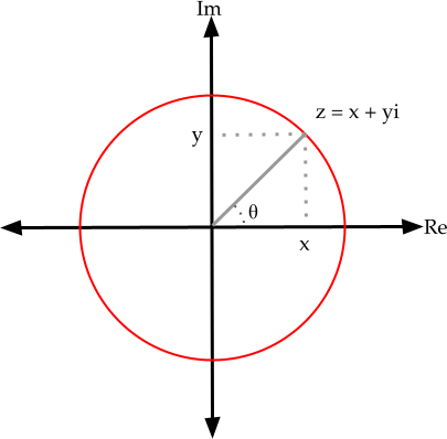
Let's verify that this works. Take the 2D vector $(x,y) = (1,1)$. If you convert this vector into a complex number, multiply by $z = e^{i\pi/4}$ using complex multiplication, and convert the result back to a 2D vector, do you get the expected result? Show your work and explain why this is the expected result.

Take a minute to convince yourself that this recipe (going from a 2D vector to a complex number, multiply by $e^{i\theta}$, and converting back to a 2D vector) is mathematically equivalent to multiplying the original number by the 2D rotation matrix: $$R(\theta) = \begin{bmatrix} \cos\theta & -\sin\theta \\ \sin\theta & \cos\theta \end{bmatrix}.$$

A frame $F$ has an orientation. We can represent that orientation using the rotation from the world frame, e.g. $^WR^F$. We've just verified that you can represent that rotation using a complex number, $e^{i\theta}$. Now assume we want to interpolate between two orientations, represented by frames $F$ and $G$. How should we smoothly interpolate between the two frames, e.g. using $t\in [0,1]$? You'll explore this in parts (b) and (c).

Attempt 1: Consider $z(t) = (a_F*(1-t) + a_G*t) + i (b_F*(1-t) + b_G*t)$. Take $t=.5$. What happens if you multiply the 2D vector $(1,1)$ by $z(t = .5)$? Show your work and explain what goes wrong.

Attempt 2: Instead we can leverage the other representation: $z(t) = e^{i \theta_{F}*(1-t) + i\theta_{G}*t}$. What happens if we multiply by the 2D vector $(1,1)$ by $z(t = .5)$? Again, show your work.

Quaternions simply are a generalization of this idea to 3D. In 2D, it might seem inefficient to use two numbers and a constraint that $a^2 + b^2 = 1$ to represent a single rotation (why not just $\theta$!?), but we've seen that it works. In 3D we can use 4 numbers $x,y,z,w$ plus the constraint that $x^2+y^2+z^2+w^2 = 1$ to represent a 3D rotation. In 2D, using just $\theta$ can work fine, but in 3D using only three numbers leads to problems like the famous gimbal lock. The 4 numbers forming a unit quaternion provides a non-degenerate mapping of all 3D rotations.

Just like we saw in 2D, one cannot simply linearly interpolate the 4 numbers of the quaternion to interpolate orientations. Instead, we linearly interpolate the angle between two orientations, using the quaternion slerp. The details involve some quaternion notation, but the concept is the same as in 2D.

Scaling spatial velocity

TODO(russt): Fill this in. Until then, here's a little code that might convince you it's reasonable.

figures/scaling_spatial_velocity.py

Planar Manipulator

For this exercise you will derive the translational forward kinematics ${^A}p{^C}=f(q)$ and the translational Jacobian $J(q)$ of a planar two-link manipulator. You will work exclusively in . You will be asked to complete the following steps:

Derive the forward kinematics of the manipulator.
Derive the Jacobian matrix of the manipulator.
Analyze the kinematic singularities of the manipulator from the Jacobian.

Exploring the Jacobian

Exercise 3.5 asked you to derive the translational Jacobian for the planar two-link manipulator. In this problem we will explore the translational Jacobian in more detail, both in the context of a planar two-link manipulator and in the context of a planar three-link manipulator. For the planar three-link manipulator, the joint angles are $(q_{0}, q_{1}, q_{2})$ and the planar end-effector position is described by $(x, y)$.

For the planar two-link manipulator, the size of the planar translational Jacobian is 2x2. What is the size of the planar translational Jacobian of the planar three-link manipulator?

In considering the planar two-link and three-link manipulators, how does the size of the translational Jacobian impact the type of inverse that can be computed? (when can the inverse be computed exactly? when can it not?)

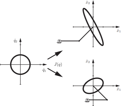
Below, for the planar two-link manipulator, we draw the unit circle of joint velocities in the $\dot{q_{1}}-\dot{q_{2}}$ plane. This circle is then mapped through the translational Jacobian to an ellipse in the end effector velocity space. In other words, this visualizes that the translational Jacobian maps the space of joint velocities to the space of end-effector velocities.

The ellipse in the end-effector velocity space is called the manipulability ellipsoid. The manipulability ellipsoid graphically captures the robot's ability to move its end effector in each direction. For example, the closer the ellipsoid is to a circle, the more easily the end effector can move in arbitrary directions. When the robot is at a singularity, it cannot generate end effector velocities in certain directions. Thinking back to the singularities you explored in Exercise 3.5, at one of these singularities, what shape would the manipulability ellipsoid collapse to?

Manipulability ellipsoids for two different postures of the planar two-link manipulator. Adapted from Lynch17.

Spatial Transforms and Grasp Pose

For this exercise you will apply your knowledge on spatial algebra to write poses of frames in different reference frames, and design a grasp pose yourself. You will work exclusively in . You will be asked to complete the following steps:

Express poses of frames in different reference frames using spatial algebra.
Design grasp poses given the configuration of the target object and griper configuration.

The Robot Painter

For this exercise you will design interesting trajectories for the robot to follow, and observe the robot virtually painting in the air! You will work exclusively in . You will be asked to complete the following steps:

Design and compute the poses of key frames of a designated trajectory.
Construct trajectories by interpolating through the key frames.

Introduction to QPs

For this exercise you will practice the syntax of solving Quadratic Programs (QPs) via Drake's MathematicalProgram interface. You will work exclusively in .

Virtual Wall

For this exercise you will implement a virtual wall for a robot manipulator, using an optimization-based approach to differential inverse kinematics. You will work exclusively in . You will be asked to complete the following steps:

Implement a optimization-based differential IK controller with joint velocity limits.
Using your own constraints, implement a virtual wall in the end-effector space using optimization-based differential IK controller.

Competing objectives

In the section on joint centering, I claimed that an secondary objective might compete with a primary objective if they are linked through constraints. To see this, consider the following optimization problem \begin{align*}\min_{x,y} \quad (x-5)^2 + (y+3)^2.\end{align*} Clearly, the optimal solution is given by $x^*=5, y^*=-3$. Moreover, the objective are separable. The addition of the second objective, $(y+3)^2$, did not in any way impact the solution of the first.

Now consider the constrained optimization \begin{align*}\min_{x,y} \quad& (x-5)^2 + (y+3)^2 \\ \subjto \quad& x - y \le 6. \end{align*} If the second objective was removed, then we would still have $x^*=5$. What is the result of the optimization as written (it's only a few lines of code, if you want to do it that way)? I think you'll find that these "orthogonal" objectives actually compete!

What happens if you change the problem to \begin{align*}\min_{x,y} \quad& (x-5)^2 + \frac{1}{100}(y+3)^2 \\ \subjto \quad& x - y \le 6? \end{align*} I think you'll find that solution is quite close to $x^*=5$, but also that $y^*$ is quite different than that $y^*=0$ one would obtain if the "secondary" objective was omitted completely.

Note that if the constraint was not active at the optimal solution (e.g. $x=5, y=-3$ satisfied the constraints), then the objectives do not compete.

This seems like an overly simple example. But I think you'll find that it is actually quite similar to what is happening in the null-space objective formulation above.

Spatial Velocity for Moving Frame

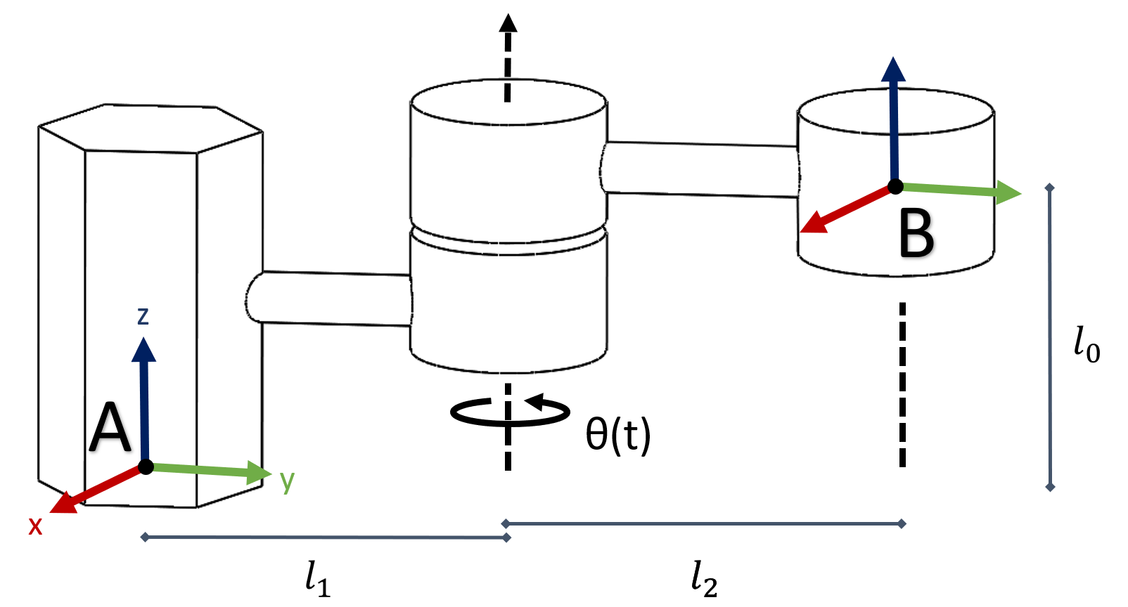
A manipulator with one moving joint. Frame A is the robot base while frame B is on the end-effector.

A manipulator with one joint is shown above. The joint is rotating over time, with its angle as a function of time, $\theta(t)$. When $t=0, \theta(t)=0$ and the link(arm) is aligned with y-axis of frame A and that of frame B. For this exercise, we will explore the spatial velocity of the end-effector.

For this manipulator, given ${}^Bp^C(0) = [1, 0, 0]^T$ , write ${}^Ap^C(0)$. For a generic point C, derive 3x3 rotation matrix ${^A}R{^B}(t)$ and translation vector ${^A}p{^B}(t)$, such that ${^A}p^C_A(t)={^A}R{^B}(t) {^B}p^C_B+{^A}p{^B} (t)$. Your solutions should involve $l_0, l_1, l_2,$ and $\theta(t)$.
Prove that for any rotation matrix $R$, $\widehat{\omega} \equiv \dot{R}R^{-1}$ satisfies $\widehat{\omega} = -\widehat{\omega}^T$. Plug in $R={^A}R{^B}(t)$ to verify your proof.
Solve for ${^A}V{^B}(t)$ for the manipulator, as a function of $l_0, l_1, l_2, \theta(t)$ and $\dot\theta(t)$.

Challenges with Representing of Rotations in 3D

In the section on representing 3D rotations, I mentioned that there is no one representation of 3D rotations that's best for everything. In this problem, you will explore some of the unexpected properties associated with a few of the most commonly used representations.

Roll-Pitch-Yaw: One way we can represent a rotation is with a set of "roll-pitch-yaw" angles $(r,p,y)$. Refer to Drake's RollPitchYaw class for conventions on the ordering of these individual angle rotations into a single rotation matrix. Given that $p=-\pi/2$, compute a rotation matrix in terms of $r$ and $y$. In the resulting matrix, how does a change in $r$ compare to a change in $y$? What does this tell us about "roll-pitch-yaw" as a representation for rotations?

Hint: Try simplifying your solution using the angle sum trigonometric identities $$\sin(\alpha+\beta)=\sin\alpha\cos\beta+\cos\alpha\sin\beta$$ $$\cos(\alpha+\beta)=\cos\alpha\cos\beta-\sin\alpha\sin\beta$$.
Axis-Angle: Consider an orientation obtained by rotating a right-handed coordinate frame about its z-axis by an angle of $\pi/2$ radians. This rotation would result in the positive x-axis pointing in the direction where the positive y-axis was pointing before rotation. One way to represent this rotation is with the axis-angles vector $(0,0,\pi/2)$. (Recall that the vector describes the axis about which the rotation occurs, and its magnitude is the angle of rotation). This representation is not unique. Find two other sets of axis-angles that would give the same rotation.
Quaternion: A unit quaternion is a set of four numbers $(w,x,y,z)$ such that $w^2+x^2+y^2+z^2=1$. Unit quaternions are an excellent way of representing orientations, since they don't suffer from singularities (unlike the roll-pitch-yaw and axis-angle representations). This makes them reliable for interpolating orientations, but unit quaternions still suffer from the "multiple representations" problem.

We can turn a unit quaternion $(w,x,y,z)$ into an axis-angle vector $(a_x,a_y,a_z)$ by computing $\theta=2\arccos(w)$, and then $$(a_x,a_y,a_z)=\left\{\begin{array}{ll} \displaystyle\frac{\theta}{\sin(\theta/2)}(x,y,z) & \theta\ne 0\\ (0,0,0) & \theta=0 \end{array}\right.$$ Show that for any unit quaternion $(w,x,y,z)$, $(-w,-x,-y,-z)$ represents the same orientation by converting to axis-angle form, and simplifying the resulting trigonometric expressions.

As it turns out, there are precisely two unit quaternions corresponding to each orientation!

Hint 1: $\arccos(-\alpha)=\pi-\arccos(\alpha)$ and $\sin(\pi-\beta)=\sin(\beta)$ for any $\alpha$ and $\beta$.
Hint 2: Use the fact that for any angle $\theta$, $\theta\pm 2\pi$ represents the same orientation.

Basic Pick and Place