Manipulator Control
Over the last few chapters, we've developed a great initial toolkit for perceiving objects (or piles of objects) in a scene, planning grasps, and moving the arm to grasp. In the last chapters, we started designing motion planning strategies that could produce beautiful smooth joint trajectories for the robot that could move it quickly from one grasp to the next. As our desired trajectories get closer to the dynamic limits of the robot, then the control strategies that we use to execute them on the robot arm also need to get a bit more sophisticated.
Remember, too, that there is a lot more to manipulation than grasping! Even in the bin picking application, we already have some examples where our grasping-only strategy can be insufficient. Imagine that you look through the robot cameras into the box and see the following scene:
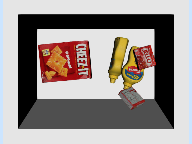
How in the world are we going to pick up that "Cheez-it" cracker box with our two-fingered gripper? (I know there are a few of you out there thinking about how easy that scene is for your suction gripper, but suction alone isn't going to solve all of our problems either.)
Click here to watch the video.
The term nonprehensile manipulation means "manipulation without grasping", and humans do it often. It is easy to appreciate this fact when we think about pushing an object that is too big to grasp (e.g. an office chair). But if you pay close attention, you will see that humans make use of strategies like sliding and environmental contact often, even when they are grasping. These strategies just come to the forefront in non-grasping manipulation.
As we build up our toolkit for prehensile (grasping) and nonprehensile manipulation, one of the things that is missing from our discussion so far, which has been predominantly kinematic, has been thinking about forces. In addition to tracking motion planning trajectories, this chapter will also introduce control techniques that reason about contact forces. I hope that by the end you'll agree that we have pretty satisfying approaches to flipping up that box!
The Manipulator-Control Toolbox
When I talk about "manipulator control", I am discussing robot controllers that take (slightly) higher-level commands, like desired joint positions and velocities or spatial forces, and convert them into motor commands. Throughout this chapter we will assume that we can command generalized forces, which for revolute-joint robots are just joint torques. These controllers, by themselves, are not enough to complete any meaningful task -- they are reasoning about the robot itself but not about any of the objects in the environment. But they facilitate writing the rest of the control systems by providing the higher-level abstraction.
Typically the low-level controllers we will be discussing here are implemented in the firmware that runs directly on the robot arm (or its control cabinet). For the purposes of using that hardware, it's important to understand how they work and how you should set their parameters. In simulation we need to implement these controllers ourselves in order to model the robot.
Drake offers a number of manipulator control implementations. In this chapter, we will work through the most relevant ones for controlling a robotic arm:
By the end of the chapter, I hope you'll understand the differences and the essentials of how they all work.
Assume your robot is a point mass
As always in our battle against complexity, I want to find a setup that
is as simple as possible (but no simpler)! Here is my proposal for the
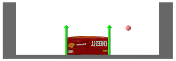
box-flipping example. First, I will restrict all motion to a 2D plane; this
allows me to chop off two sides of the bin (for you to easily see inside),
but also drops the number of degrees of freedom we have to consider. In
particular, we can avoid the quaternion floating base coordinates, by adding
a PlanarJoint to the box. Instead of using a complete gripper,
let's start even simpler and just use a "point finger". I've visualized it
as a small sphere, and modeled two control inputs as providing force
directly on the $x$ and $z$ coordinates of the point mass.
Even in this simple model, and throughout the discussions in this chapter, we will have two dynamic models that we care about. The first is the full dynamic model used for simulation: it contains the finger, the box, and the bin, and has a total of 5 degrees of freedom ($x, z, \theta$ for the box and $x, z$ for the finger). The second is the robot model used for designing the controllers: this model has just the two degrees of freedom of the finger, and experiences unmodelled contact forces. By design, the equations of this second model are particularly simple: $$\begin{bmatrix}m & 0 \\ 0 & m \end{bmatrix} \dot{v} = m \begin{bmatrix}\ddot{x} \\ \ddot{z} \end{bmatrix} = \tau_g + \begin{bmatrix} u_x \\ u_z \end{bmatrix} + f^{F_c},$$ where $m$ is the mass, $\tau_g$ is the gravitational "torque" which here is just $\tau_g = [0, -mg]^T$, $u$ is the control input vector, and $f^{F_c}$ is the Cartesian contact force applied to the finger, $F$, at $c$.
This chapter will make heavy use of our spatial force notation. To make sure it's clear, I've used $f^{F_c}$ above to denote force applied to the finger, $F$, at point $c$. If we want to denote the same force applied to the box, $B$, at point $c$, then we'll denote it as $f^{B_c}$. Naturally, we have $f^{F_c} = - f^{B_c}$, because the forces must be equal and opposite. If we're not careful about this notation, the signs will definitely get confusing below.
Trajectory tracking
Before we even make contact with the box, let's make sure we know how to move our robot finger around through the air. Assume that you've done some motion planning, perhaps using optimization, and have developed a beautiful desired trajectory, $q_d(t)$, that you want your finger to follow. Let's assume that $q_d(t)$ is twice differentiable. What generalized-force commands should you send to the robot to execute that trajectory?
One of the first and most common ways to execute the trajectory is with proportional-integral-derivative (PID) control, which we've discussed when we talked about position-controlled robots. The PidController uses the command $$u(t) = K_p (q_d(t) - q(t)) + K_d (\dot{q}_d(t) - \dot{q}(t)) + K_i \int_0^t (q_d(t) - q(t)) dt,$$ with $K_p$, $K_d$, and $K_i$ being the position, velocity, and integral gains. Often these gains are diagonal matrices, making the command for each joint independent of the rest. Note that in manipulation, we tend to avoid the integral term, setting $K_i = 0$. You can imagine that if the robot is pushing up against the wall and is unable to achieve $q(t) == q_d(t)$, then the integral term will "wind-up", sending larger and larger commands to the robot until some fault is reached.
PD control can be incredibly effective; it assumes almost nothing
about the dynamics of the robot. But this assumption is also a
limitation; if we do know something about the dynamics of the robot then
we can achieve better tracking performance. To make that clear, let's
write the closed-loop dynamics of the $z$ position of our robot finger
under PD control:$$m \ddot{z} = -mg + k_p (z_d - z) + k_d (\dot{z}_d -
\dot{z}).$$ Here is a sample roll-out when we command a sinusoidal
trajectory, $z_d(t)$, and start the finger slightly off the trajectory in
$z$ and $\dot{z}$:

Looking at the equations, it seems clear that we can do better if we inform the controller about the gravity term. This is commonly referred to as "gravity compensation". For reasons that will become clear soon, the gravity compensation + PD controller is available in Drake as the JointStiffnessController, $$u = -\tau_g + K_p (q_d - q) + K_d (\dot{q}_d - \dot{q}).$$ For the $z$ axis of our point finger, this results in the closed-loop dynamics: $$m \ddot{z} = k_p (z_d - z) + k_d (\dot{z}_d - \dot{z}).$$ This controller has no steady-state error, and tracks better in practice:

Although the steady-state error is gone, we can still see errors when
tracking a more complicated desired trajectory. There is one more
relevant piece of information, however, which we have access to, but
which we have not yet given to our controller: $\ddot{q}_d(t)$. Let's
write our controller access in a subtly different form: $$u = -\tau_g +
m\left[\ddot{q}_d + K_p (q_d - q) + K_d (\dot{q}_d - \dot{q}) \right].$$
The general form of this controller is available in Drake as the InverseDynamicsController.
Two things changed here; in addition to adding the feed-forward
acceleration term into the controller, we also multiplied the PD terms by
the mass. Combined, this has the result that the closed-loop error
dynamics simplifies to $$\ddot{\tilde{z}} + k_d \dot{\tilde{z}} + k_p
\tilde{z} = 0,$$ which may be familiar to you as a simple
mass-spring-damper model. Given reasonable choices for $k_p$ and $k_d$,
the error dynamics converge nicely to zero, giving us our best tracking
performance yet:

Trajectory tracking for the point mass
I've put the code to generate these simple plots into a notebook so that you can play around with them yourself:
(Direct) force control
Things get more interesting when we start making contact (in our example, it means our finger starts contacting the box). In this case, controlling the position / velocity / acceleration of the finger might not be the only goal. We might also want to control the interaction forces that we are applying to the box.
In the simplest case, let's not try to regulate the finger position at all, but instead implement a low-level controller that accepts the desired contact forces and produces generalized force inputs to the robot that try to make the actual contact forces match the desired.
What information do we need to regulate the contact forces? Certainly we need the desired contact force, $f^{F_c}_{desired}$. In general, we will need the robot's state (though in the immediate example, the dynamics of our point mass are not state dependent). But we also need to either (1) measure the robot accelerations (which we've try to avoid, since they are often noisy measurements), (2) assume the robot accelerations are zero, or (3) provide a measurement of the contact force so that we can regulate it with feedback.
Let's consider the case where the robot is already in contact with the box. Let's also assume for a moment that the accelerations are (nearly) zero. This is actually not a horrible assumption for most manipulation tasks, where the movements are relatively slow. In this case, our equations of motion reduce to $$f^{F_c} = - mg - u.$$ Our force controller implementation can be as simple as $u = -mg - f^{F_c}_{desired}.$ Note that we only need to know the mass of the robot (not the box) to implement this controller.
What happens when the robot is not in contact? In this case, we cannot reasonably ignore the accelerations, and applying the same control results in $m\dot{v} = - f^{F_c}_{desired}.$ That's not all bad. In fact, it's one of the defining features of force control that makes it very appealing. When you specify a desired force and don't get it, the result is accelerating the contact point in the (opposite) direction of the desired force. In practice, this (locally) tends to bring you into contact when you are not in contact.
Commanding a constant force
Let's see what happens when we run a full simulation which includes not only the non-contact case and the contact case, but also the transition between the two (which involves collision dynamics). I'll start the point finger next to the box, and apply a constant force command requesting to get a horizontal contact force from the box. I've drawn the $x$ trajectory of the finger for different (constant) contact force commands.

For all strictly positive desired force commands, the finger will accelerate at a constant rate until it collides with the box (at $x=0.089$). For small $f^{F_c}_{desired}$, the box barely moves. For an intermediate range of $f^{F_c}_{desired}$, the collision with the box is enough to start it moving, but friction eventually brings the box and therefore also the finger to rest. For large values, the finger will keep pushing the box until it runs into the far wall.
Consider the consequences of this behavior. By commanding force, we can write a controller that will come into a nice contact with the box with essentially no information about the geometry of the box (we just need enough perception to start our finger in a location for which a straight-line approach will reach the box).
This is one of the reasons that researchers working on legged robots also like force control. On a force-capable walking robot, we might mimic position control during the "swing phase", to get our foot approximately where we are hoping to step. But then we switch to a force control mode to actually set the foot down on the ground. This can significantly reduce the requirements for accurate sensing of the terrain.
A force-based flip-up strategy
Here is my proposal for a simple strategy for flipping up the box. Once in contact, we will use the contact force from the finger to apply a moment around the bottom left corner of the box to generate the rotation. But we'll add constraints to the forces that we apply so that the bottom corner does not slip.
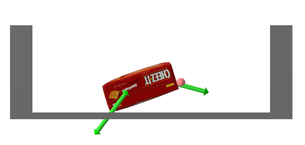
These conditions are very natural to express in terms of forces. And once again, we can implement this strategy with very little information about the box. The position of the finger will evolve naturally as we apply the contact forces. It's harder for me to imagine how to write an equally robust strategy using a (high-gain) position-controller finger; it would likely require many more assumptions about the geometry (and possibly the mass) of the box.
Let's encode the textual description above, describing the forces that are applied to the box. I'll use $C$ for the contact frame between the finger and the box, with its normal pointing into the box normal to the surface, and $A$ for the contact frame for the lower left corner of the box contacting the bin, with the normal pointing straight up in positive world $z$. $${}^BR^C = R_y(-\frac{\pi}{2}), \qquad {}^WR^A = I,$$ where $R_y(\theta)$ is a rotation by $\theta$ around the y axis. Of course we also have the force of gravity, which is applied at the body center of mass (com): $$f^{B_{com}}_{gravity,W} = mg.$$ As you can see, we'll make heavy use of the spatial force notation / spatial algebra described here.
The friction cone provides (linear inequality) constraints on the forces we want to apply. \begin{gather*} f^{B_C}_{\text{finger}, C_z} \ge 0, \qquad |f^{B_C}_{\text{finger}, C_x}| \le \hat\mu_C f^{B_C}_{\text{finger}, C_z}, \\ f^{B_A}_{\text{ground}, A_z} \ge 0, \qquad |f^{B_A}_{\text{ground}, A_x}| \le \hat\mu_A f^{B_A}_{\text{ground}, A_z}.\end{gather*} Please make sure you understand the notation. Within those constraints, we would like to rotate up the box.
To rotate the box about $A$, let's reason about the total torque being applied about $A$: $$\tau^{B_A}_{total,W} = \tau^{B_A}_{gravity, W} + \tau^{B_A}_{ground, W} + \tau^{B_A}_{finger, W},$$ but we know that $\tau^{B_A}_{ground, W} = 0$ since the moment arm is zero. I have a goal here of not making too many assumptions about the mass and geometry of the box in our controller, so rather than try to regulate this torque perfectly, let's write $$\tau^{B_A}_{total,W_y} = \tau^{B_A}_{finger,W_y} + \text{unknown terms}.$$ A reasonable control strategy in the face of these unmodeled terms is to use feedback control on the angle of the box (call it $\theta$) which is the $y$ component of ${}^WR^B$: $$ \tau^{B_A}_{finger_d,W_y} = \text{PID}(\theta_d, \theta), \qquad {}^WR^B(\theta) = R_y(\theta),$$ where I've used $\theta_{d}$ as shorthand for the desired box angle and $\text{PID}$ as shorthand for a simple proportional-integral-derivative term. Note that $\tau^{B_A}_{finger,W_y} \propto f^{B_C}_{finger, C_x},$ where the (constant) coefficient only depends on ${}^B\hat{p}^C;$ it does not actually depend on $\hat\theta.$
To execute the desired PID control subject to the friction-cone constraints, we can use constrained least-squares: \begin{align*}\min_{f^{B_C}_{finger,C}, \, f^{B_A}_{ground,A}} \quad& \left| \tau^{B_A}_{finger,W_y} - \text{PID}(\theta_d, \hat\theta) \right|^2,\\ \subjto \quad & f^{B_C}_{\text{finger}, C_z} \ge 0, \qquad |f^{B_C}_{\text{finger}, C_x}| \le \hat\mu_C f^{B_C}_{\text{finger}, C_z}, \\ & f^{B_A}_{\text{ground}, A_z} \ge 0, \qquad |f^{B_A}_{\text{ground}, A_x}| \le \hat\mu_A f^{B_A}_{\text{ground}, A_z}, \\ & f^{B_A}_{\text{ground}, A} + \hat{f}^{B_A}_{gravity, A} + f^{B_A}_{finger, A} = 0.\end{align*} Note that the last line is still a linear constraint once $\hat\theta$ is given, despite requiring some spatial algebra operations. Implementing this strategy assumes:
- We have some approximation, $\hat\theta$, for the orientation of the box. We could obtain this from a point cloud normal estimation, or even from tracking the path of the fingers.
- We have conservative estimates of the coefficients of static friction between the wall and the box, $\hat\mu_A$, and between the finger and the box, $\hat\mu_C$, as well as the approximate location of the finger relative to the box corner, and the box mass, $\hat{m}.$
We have multiple controllers in this example. The first is the low-level force controller that takes a desired contact force and sends commands to the robot to attempt to regulate this force. The second is the higher-level controller that is looking at the orientation of the box and deciding which forces to request from the low-level controller.
Please also understand that this is not some unique or optimal strategy for box flipping. I'm simply trying to demonstrate that sometimes controllers which might be difficult to express otherwise can easily be expressed in terms of forces!
Indirect force control
There is a nice philosophical alternative to controlling the contact
interactions by specifying the forces directly. Instead, we can program
our robot to act like a (simple) mechanical system that reacts to contact
forces in a desired way. This philosophy was described nicely in an
important series of papers by Ken Salisbury introducing stiffness
control
This approach is conceptually very nice. Imagine we were to walk up and push on the end-effector of the iiwa. With only knowledge of the parameters of the robot itself (not the environment), we can write a controller so that when we push on the end-effector, the end-effector pushes back (using the entire robot) as if you were pushing on, for instance, a simple spring-mass-damper system. Rather than attempting to achieve manipulation by moving the end-effector rigidly through a series of position commands, we can move the set points (and perhaps stiffness) of a soft virtual spring, and allow this virtual spring to generate our desired contact forces.
This approach can also have nice advantages for guaranteeing that your
robot won't go unstable even in the face of unmodeled contact
interactions. If the robot acts like a dissipative system and the
environment is a dissipative system, then the entire system will be
stable. Arguments of this form can ensure stability for even very complex
system, building on the rich literature on passivity theory or more
generally Port-Hamiltonian
systems
Our simple model with a point finger is ideal for understanding the essence of indirect force control. The original equations of motion of our system are $$m\begin{bmatrix}\ddot{x} \\ \ddot{z} \end{bmatrix} = mg + u + f^{F_c}.$$ We can write a simple controller to make this system act, instead, like (passive) mass-spring-damper system: $$m \begin{bmatrix}\ddot{x} \\ \ddot{z} \end{bmatrix} + b \begin{bmatrix} \dot{x} \\ \dot{z} \end{bmatrix} + k \begin{bmatrix} x - x_d \\ z - z_d \end{bmatrix} = f^{F_c},$$ with the rest position of the spring at $(x_d, z_d).$ The controller that implements this follows easily; in the point finger case this has the familiar form of a proportional-derivative (PD) controller, but with an additional "feed-forward" term to cancel out gravity.
Technically, if we are just programming the stiffness and damping, as I've written here, then a controller of this form would commonly be referred to as "stiffness control", which is a subset of impedance control. We could also change the effective mass of the system; this would be impedance control in its full glory. My impression, though, is that the consensus in robot control experts is that changing the effective mass is most often considered not worth the complexity that comes from the extra sensing and bandwidth requirements.
The literature on indirect force control has a lot of terminology and
implementation details that are important to get right in practice. Your
exact implementation will depend on, for instance, whether you have access
to a force sensor and whether you can command forces/torque directly. The
performance can vary significantly based on the bandwidth of your
controller and the quality of your sensors. See e.g.
Teleop with stiffness control
I didn't give you a teleop interface with direct force control; it would have been very difficult to use! Moving the robot by positioning the set points on virtual springs, however, is quite natural. Take a minute to try moving the box around, or even flipping it up.
To help your intuition, I've made the bin and the box slightly transparent, and added a visualization (in orange) of the virtual finger or gripper that you are moving with the sliders.
Let's embrace indirect force control to come up with another approach to flipping up the box. Flipping the box up in the middle of the bin required very explicit reasoning about forces in order to stay inside the friction cone in the bottom left corner of the box. But there is another strategy that doesn't require as precise control of the forces. Let's push the box into the corner, and then flip it up.
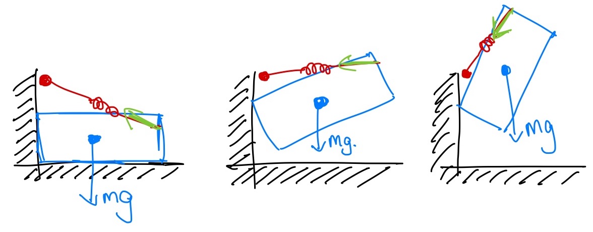
To make this one happen, I'd like to imagine creating a virtual spring -- you can think of it like a taut rubber band -- that we attach from the finger to a point near the wall just a little above the top left corner of the box. The box will act like a pendulum, rotating around the top corner, with the rubber band creating the moment. At some point the top corner will slip, but the very same rubber band will have the finger pushing the box down from the top corner to complete the maneuver.
Consider the alternative of writing an estimator and controller that needed to detect the moment of slip and make a new plan. That is not a road to happiness. By only using our model of the robot to make the robot act like a different dynamical system at the point we can accomplish all of that!
A stiffness-control-based flip-up strategy
This controller almost couldn't be simpler. I will just command a trajectory the move the virtual finger to just in front of the wall. This will push the box into contact and establish our bracing contact force. Then I'll move the virtual finger (the other end of our rubber band) up the wall a bit, and we can let mechanics take care of the rest!
So far we've made our finger act like two independent mass-spring-damper systems, one in $x$ and the other in $z$. We even used the same stiffness, $k$, and damping, $b$, parameters for each. More generally, we can write stiffness and damping matrices, which we typically would call $K_p$ and $K_d$, respectively: $$m \begin{bmatrix}\ddot{x} \\ \ddot{z} \end{bmatrix} + K_d \begin{bmatrix} \dot{x} \\ \dot{z} \end{bmatrix} + K_p \begin{bmatrix} x - x_d \\ z - z_d \end{bmatrix} = f^{F_c}.$$ In order to emphasize the coordinate frame of these stiffness matrices, let's write exactly the same equation, realizing that with our point finger we have ${}^Wp^F = \begin{bmatrix} x, z\end{bmatrix}^T,$ so: $$m\,{}^W\dot{v}^F + K_d \, {}^Wv^F + K_p\left({}^Wp^F - {}^Wp^{F_d}\right) = f^F.$$ Sometimes it can be convenient to express the stiffness (and/or damping) matrices in a different frame, $A$: \begin{align*} m\,{}^W\dot{v}^F + {}^W R^A K_d \, {}^Wv^F_A + {}^WR^W K_p\left({}^Wp^F_A - {}^Wp^{F_d}_A\right) =& \\ m\,{}^W\dot{v}^F + {}^W R^A K_d {}^A R^W\, {}^Wv^F + {}^WR^A K_p {}^A R^W\left(\,{}^Wp^F - {}^Wp^{F_d}\right) =& \, f^F.\end{align*}
Hybrid position/force control
There are a number of applications where we would like to explicitly command force in one direction, but command positions in another. One classic examples if you are trying to wipe or polish a surface -- you might care about the amount of force you are applying normal to the surface, but use position feedback to follow a trajectory in the directions tangent to the surface. In the simplest case, imagine controlling force in $z$ and position in $x$ for our point finger: $$u = -mg + \begin{bmatrix} k_p (x_d - x) + k_d (\dot{x}_d - \dot{x}) \\ -f^F_{desired, W_z} \end{bmatrix}.$$ If want the forces/positions in a different frame, for instance the contact frame, $C$, then we can use \begin{equation} u = -mg + {}^WR^C \begin{bmatrix} k_p (p^{F_d}_{C_x} - p^{F}_{C_x}) + k_d (v^{F_d}_{C_x} - v^F_{C_x}) \\ -f^{F}_{desired, C_z}\end{bmatrix}. \label{eq:position-or-force}\end{equation} By commanding the normal force, you not only have the benefit of controlling how hard the robot is pushing on the surface, but also gain some robustness to errors in estimating the surface normal. If a position-controlled robot estimated the normal of a wall badly, then it might leave the wall entirely in one direction, and push extremely hard in the other. Having a commanded force in the normal direction would allow the position of the robot in that direction to become whatever is necessary to apply the force, and it will follow the wall.
Click here to watch the video.
The choice of position control or force control need not be a binary decision. We can simply apply both the position command (as in stiffness/impedance control) and a "feed-forward" force command: $$u = -mg + K_p (p^{F_d} - p^{F}) + K_d (v^{F_d} - v^{F}) - f^{F}_{\text{feedforward}}.$$ Certainly this is only more general that the explicit position-or-force mode in Eq. (\ref{eq:position-or-force}); we could achieve the explicit position-or-force in this interface by the appropriate choices of $K_p$, $K_d$, and $f^F_{feedforward}.$ As we'll see, this is quite similar to the interface provided by the iiwa (and many other torque-controlled robots).
The general case (using the manipulator equations)
Using the floating finger/gripper is a good way to understand the main concepts of force control without the details. But now it's time to actually implement those strategies using joint commands that we can send to the arm.
Our starting point is understanding that the equations of motion for a fully-actuated robotic manipulator have a very structured form: \begin{equation}M(q)\ddot{q} + C(q,\dot{q})\dot{q} = \tau_g(q) + u + \sum_i J^T_i(q)f^{c_i}.\label{eq:manipulator} \end{equation} The left side of the equation is just a generalization of "mass times acceleration", with the mass matrix, $M$, and the Coriolis terms $C$. The right hand side is the sum of the (generalized) forces, with $\tau_g(q)$ capturing the forces due to gravity, $u$ the joint torques supplied by the motors, and $f^{c_i}$ is the Cartesian force due to the $i$th contact, where $J_i(q)$ is the $i$th "contact Jacobian". I introduced a version of these briefly when we described multibody dynamics for dropping random objects into the bin, and have more notes available here. For the purposes of the remainder of this chapter, we can assume that the robot is bolted to the table, so does not have any floating joints; I've therefore used $\dot{q}$ and $\ddot{q}$ instead of $v$ and $\dot{v}$.
Trajectory tracking
Let us ignore the contact terms for a moment: $$M(q)\ddot{q} + C(q,\dot{q})\dot{q} = \tau_g(q) + u.$$ The forward dynamics problem, which we use during simulation, is to compute the accelerations, $\ddot{q}$, given the joint torques, $u$, (and $q, \dot{q}$). The inverse dynamics problem, which we can use in control, is to compute $u$ given $\ddot{q}$ (and $q, \dot{q}$). As a system, it looks like
This system implements the controller: $$u = M(q)\ddot{q}_d + C(q,\dot{q})\dot{q} - \tau_g(q),$$ so that the resulting dynamics are $M(q)\ddot{q} = M(q)\ddot{q}_d.$ Since we know that $M(q)$ is invertible, this implies that $\ddot{q} = \ddot{q}_d$.
When we put the contact forces back in, In practice, we only have estimates of the dynamics (mass matrix, etc) and even the states $q$ and $\dot{q}$. We will need to account for these errors when we determine the acceleration commands to send. For example, if we wanted to follow a desired joint trajectory, $q_0(t)$, we do not just differentiate the trajectory twice and command $\ddot{q}_0(t)$, but we could instead command e.g. $$\ddot{q}_d = \ddot{q}_0(t) + K_p(q_0(t) - q) + K_d(\dot{q}_0(t) - \dot{q}).$$ One could also include an integral gain term.
The resulting System has one additional input port for the desired state:
This "inverse dynamics control" also appears in the literature with a
few other names, such as "computed-torque control" and even the
"feedforward-plus-feedback-linearizing control"
Check yourself: What is the difference between the joint stiffness control and the inverse dynamics control?
The closed-loop dynamics with the joint stiffness control (taking $\tau_{ff} = 0$) are given by $$M(q)\ddot{q} + C(q,\dot{q})\dot{q} + K_p(q - q_d) + K_d(\dot{q} - \dot{q}_d) = \tau_{ext},$$ where $\tau_{ext}$ summarized the results of (unmodeled) forces like contacts. The closed-loop dynamics with the inverse dynamics controllers are given by $$\ddot{q} + K_p(q - q_d) + K_d(\dot{q} - \dot{q}_d) = M^{-1}(q) \tau_{ext}.$$ So the inverse dynamics controller writes the feedback law in the units of accelerations rather than forces; this would be similar to shaping the internal matrix into the diagonal matrix.
The ability to realize this cancellation in hardware, however, will be limited by the accuracy with which we estimate the model parameters, $\hat{M}(q)$ and $\hat{C}(q,\dot{q})$. The stiffness controller, on the other hand, achieves much of the desired performance but only attempts to cancel the gravity (and perhaps friction) terms; it does not shape the inertia.
Joint stiffness control
In practice, the way that we most often interface with the iiwa is
through the its "joint-impedance control" mode, which is written up
nicely in
Check yourself: What is the difference between traditional position control with a PD controller and joint-stiffness control?
The difference in the algebra is quite small. A PD control would typically have the form $$u=K_p(q_d-q) + K_d(\dot{q}_d - \dot{q}),$$ whereas stiffness control is $$u = -\tau_g(q) + K_p(q_d-q) + K_d(\dot{q}_d - \dot{q}).$$ In other words, stiffness control tries to cancel out the gravity and any other estimated terms, like friction, in the model. As written, this obviously requires an estimated model (which we have for iiwa, but don't believe we have for most arms with large gear-ratio transmissions) and torque control. But this small difference in the algebra can make a profound difference in practice. The controller is no longer depending on error to achieve the joint position in steady state. As such we can turn the gains way down, and in practice have a much more compliant response while still achieving good tracking when there are no external torques.
Cartesian stiffness and operational space control
A better analogy for the control we were doing with the point finger
example is to write a controller so that the robot acts like a simple
dynamical system in the world frame. To do that, we have to identify a
frame, $E$ for "end-effector", on the robot where we want to impose these
simple dynamics -- ideally the origin of this frame will be the expected
point of contact with the environment. Following our treatment of kinematics
and differential kinematics, we'll
define the forward kinematics of this frame as: \begin{equation}p^E =
f_{kin}(q), \qquad v^E = \dot{p}^E = J(q) \dot{q}, \qquad a^E =
\ddot{p}^E = J(q)\ddot{q} + \dot{J}(q)
\dot{q}.\label{eq:kinematics}\end{equation} We haven't actually written
the second derivative before, but it follows naturally from the chain
rule. Also, I've restricted this to the Cartesian positions for
simplicity; one can think about the orientation of the end-effector, but
this requires some care in defining the 3D stiffness in orientation (e.g.
One of the big ideas from manipulator control is that we can actually write the dynamics of the robot in the frame $E$, by parameterizing the joint torques as a translational force applied to body $B$ at $E$, $f^{B_E}_u$: $u = J^T(q) f^{B_E}_u$. This comes from the principle of virtual work. By substituting this and the manipulator equations (\ref{eq:manipulator}) into (\ref{eq:kinematics}) and assuming that the only external contacts happen at $E$, we can write the dynamics: \begin{equation} M_E(q) \ddot{p}^E + C_E(q,\dot{q})\dot{q} = f^{B_E}_g(q) + f^{B_E}_u + f^{B_E}_{ext} \label{eq:cartesian_dynamics},\end{equation} where $$M_E(q) = (J M^{-1} J^T)^{-1}, \qquad C_E(q,\dot{q}) = M_E \left(J M^{-1} C - \dot{J} \right), \qquad f^{B_E}_g(q) = M_E J M^{-1} \tau_g.$$ Now if we simply apply a controller analogous to what we used in joint space, e.g.: $$f^{B_E}_u = -f^{B_E}_g(q) + K_p(p^{E_d} - p^E) + K_d(\dot{p}^{E_d} - \dot{p}^E),$$ then we can achieve the desired closed-loop dynamics at the end-effector: $$M_E(q) \ddot{p}^E + C_E(q,\dot{q})\dot{q} + K_p(p^{E} - p^{E_d}) + K_d(\dot{p}^{E} - \dot{p}^{E_d}) = f^{B_E}_{ext}.$$ So if I push on the robot at the end-effector, the entire robot will move in a way that will make it feel like I'm pushing on a spring-damper system. Beautiful!
When $J(q)$ can be rank-deficient (for instance, if you have more
degrees of freedom than you are trying to control at the end-effector),
you'll also want to add some terms to similar to
stabilize the null space of your
Jacobian. Since we are operating here with torques instead of
velocity commands, the natural analogue is to write the a joint-centering
PD controller that operates in the null space of the end-effector control:
$$u = J^Tf^{B_E}_u + P[K_{p,joint} (q_0 - q) - K_{d,joint}\dot{q}].$$
Here $P$ is the so-called "dynamically-consistent null-space projection"
This approach of programming the task-space dynamics with
secondary joint-space objectives operating in the null space was developed
in
Some implementation details on the iiwa
The implementation of the low-level impedance controllers has many
details that are explained nicely in
The iiwa interface offers a Cartesian impedance control mode. If we want high performance stiffness control in end-effector coordinates, then we should definitely use it! The iiwa controller runs at a much higher bandwidth (faster update rate) than the interface we have over the provided network API, and many implementation details that they have gone to great lengths to get right. But in practice we do not use it, because we cannot convert between joint impedance control and Cartesian impedance control without shutting down the robot. Sigh. In fact we cannot even change the stiffness gains nor the frame $C$ (aka the "end-effector location") without stopping the robot. So we stay in joint impedance mode and command some Cartesian forces through $\tau_{ff}$ if we desire them. (If you are interested in the driver details, then I would recommend the documentation for the Franka Control Interface which is much easier to find and read, and is very similar to functionality provided by the iiwa driver.)
You might also notice that the interface we provide to the
IiwaDriver in the HardwareStation takes a
desired joint position for the robot, but not a desired joint velocity.
That is because we cannot actually send a desired joint velocity to the
iiwa controller. In practice, we believe that they are numerically
differentiating our position commands to obtain the desired velocity,
which adds a delay of a few control timesteps (and sometimes non-monotonic
behavior). I believe that the reason why we aren't allowed to send
our own joint velocity commands is to to make the passivity argument in
their paper go through, and perhaps to make a simpler/safer API -- they
don't want users to be able to send a series of inconsistent position and
velocity commands (where the velocities are not actually the time
derivatives of the positions).
Since the controller attempts to cancel gravitational terms, one can also tell the iiwa firmware about the lumped inertia of the gripper. This is set just once (in the pendant), and cannot be changed while the robot is moving; if you pick something up (or even move the fingers), those changes in the gravitational terms will not be compensated in the controller.
Although the JointStiffnessController in Drake is the best model for the iiwa control stack, we commonly use the InverseDynamicsController in our simulations instead. This is for a fairly subtle reason -- the numerics are better. The effective stiffness of the differential equations to achieve comparable stiffness in the physics is smaller, and one can take bigger integration timesteps. On the iiwa hardware, we commonly use [800., 600, 600, 600, 400, 200, 200] Nm/rad as the stiffness values for the JointStiffnessController; but simulating with those requires small integration steps.
Putting it all together
Peg in hole
One of the classic problems for manipulator force control, inspired by robotic assembly, is the problem of mating two parts together under tight kinematic tolerances. Perhaps the cleanest and most famous version of this is the problem of inserting a (round) peg into a (round) hole. If your peg is square and your hole is round, I can't help. Interestingly, much of the literature on this topic in the late 1970's and early 1980's came out of MIT and the Draper Laboratory.
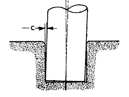
For many peg insertion tasks, it's acceptable to add a small chamfer to the part and/or the top of the hole. This allows small errors in horizontal alignment to be accounted for with a simple compliance in the horizontal direction. Misalignment in orientation is even more interesting. Small misalignments can cause the object to become "jammed", at which point the frictional forces become large and ambiguous (under the Coulomb model); we really want to avoid this. Again, we can avoid jamming by allowing a rotational compliance at the contact. I think you can see why this is a great example for force control!
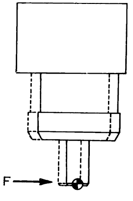
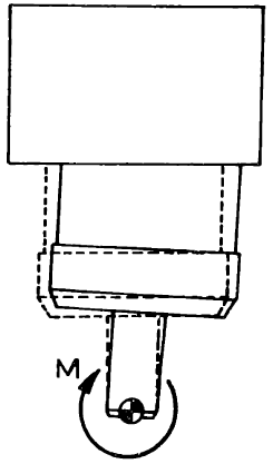
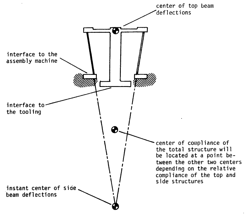
The key insight here is that the rotational stiffness that we want
should result in rotations around the part/contact, not around the gripper.
We can program this with stiffness control; but for very tight tolerances
the sensing and bandwidth requirements become a real limitation. One of
the coolest results in force control is the realization that a clever
physical mechanism can be used to produce a "remote-centered compliance"
(RCC) completely mechanically, with infinite bandwidth and no sensing
required

Interestingly, the peg-in-hole problem inspired incredibly important
and influential ideas in mechanics and control, but also in motion planning
Exercises
Force and Position Control
Suppose you are given a point-mass system with the following dynamics:
$$m\ddot{x} = u + f^{F_c}$$where $x$ is the position, $u$ the input force applied on the point-mass, and $f^{F_c}$ the contact force from the environment on point ${F}$ applied at $c$. In order to control the position and force from the robot at the same time, the following controller is proposed:
$$u = \underbrace{k_p(x_d-x) - k_d\dot{x}}_{\text{feedback force for position control}} - \underbrace{f^{F_c}_{desired}}_{\text{feedforward force}}$$Define the error for this system to be:
$$e = (x - x_d)^2 + (f^{F_c} - f^{F_c}_{desired})^2$$- Let's consider the case where our system is in free space (i.e. $f^{F_c}=0$) and we want to exert a non-zero desired force ($f^{F_c}_{desired} \neq 0$) and drive our position to zero ($x_d = 0$). You will show that this is not possible, i.e. we cannot achieve zero error for our desired force and desired position. You can show this by considering the steady-state error (i.e. set $\dot{x}=0,\ddot{x}=0$) as a function of the system dynamics, controller, desired position and desired force.
- Now consider the system is in rigid body contact with a wall located at $x_d = 0$ and a desired non-zero force ($f^{F_c}_{desired} > 0$) is being commanded. Considering the steady-state error in this case, show that system can achieve zero error.
Box Flip-up
Consider the initial phase of the box flip-up task from the example above, when $\theta\approx 0$. Let $B$ be the box, $A$ be the pivot point of the box, and $C$ be the contact point between the finger and box $B$. We will assume that the forces can still be approximated as axis-aligned, but the ground contact is only being applied at the pivoting point $A$.
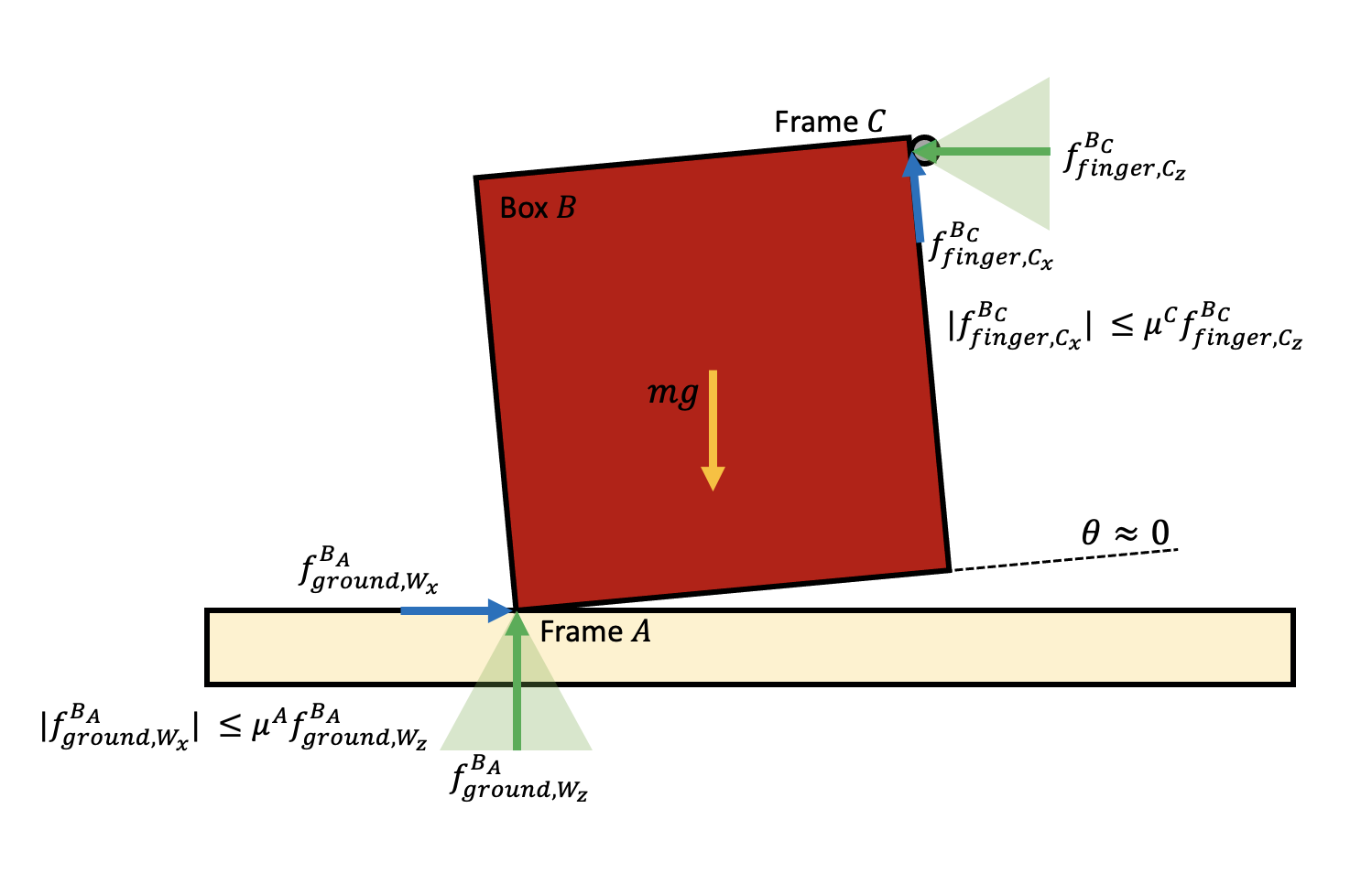
- If we do not push hard enough (i.e. $f^{C}_{finger,z}$ is too small), then we will not be able to create enough friction ($f^{C}_{finger,x}$) to counteract gravity. By summing the torques around the pivot point $A$ to obtain $\tau^{A}_{\text{total}, y}$, derive a lower bound for the required normal force $f^{C}_{finger,z}$, as a function of $m,g,$ and $\mu^C$. You may assume the box is square and that the moment arm of gravity is half the moment arm on C.
- If we push too hard (i.e. $f^{C}_{finger,z}$ is too big), then the pivot point will slide to the left. First, balance forces along the horizontal axis to derive an upper bound for $f^{C}_{finger, z}$. Then, balance forces along the y-axis to obtain an equation with $f^{C}_{finger,z}$. Finally, combine the relations found from balancing forces in the horizontal and vertical directions with the torque lower bound from part (a) to finish deriving the upper bound for the required normal force $f^{C}_{finger,z}$ as a function of $m,g,$ and $\mu^A$. (Assume $\mu^A < 1$ and that we have achieved a positive $\tau^{A}_{\text{total},y}.$)
- By combining the lower bounds and upper bounds from the previous problems, derive a relation for $\mu^A,\mu^C$ that must hold in order for this motion to be possible. If $\mu^A\approx 0.25$ (wood-metal), how high does $\mu^C$ have to be in order for the motion to be feasible? What if $\mu^A=1$ (concrete-rubber)?
Hybrid Force-Position Control
For this exercise, you will analyze and implement a hybrid force-position controller to drag a book, as we saw from this video during lecture. You will work exclusively in . You will be asked to complete the following steps:
- Analyze the conditions for this motion to be feasible.
- Implement a control law to implement the motion
Peg-in-hole control
In this exercise you will play with the peg-in-hole task for robotic manipulation. Specifically, you will gain experience with indirect force control through implementing two different stiffness controllers. You will work exclusively in . You will be asked to complete the following steps:
- Implement stiffness control for a floating peg (where configuration and task-space are the same).
- Implement an operational space stiffness controller for the full planar iiwa.